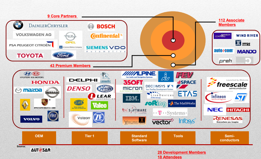
AUTOSAR (AUTomotive Open System ARchitecture) is a worldwide development partnership of automotive manufacturers, suppliers, and other companies in the electronics, semiconductor, and software industries. AUTOSAR standards are designed for software standardization, reuse, and interoperability.
AUTOSAR has implemented a layered architecture similar to OSI model. It has different layers to handle and abstract different operations of code.
The AUTOSAR standard provides two platforms to support current and future generations of automotive electronic control units (ECUs).
The Classic Platform supports traditional internal applications such as powertrain, chassis, body, and interior electronics.
The Adaptive Platform supports service-based applications such as autonomous driving, Car-to-X, over-the-air (OTA) software updates, and using vehicles as part of the Internet of Things (IoT).
AUTOSAR Classic, AUTOSAR Adaptive, and non-AUTOSAR ECUs can interoperate in one vehicle.
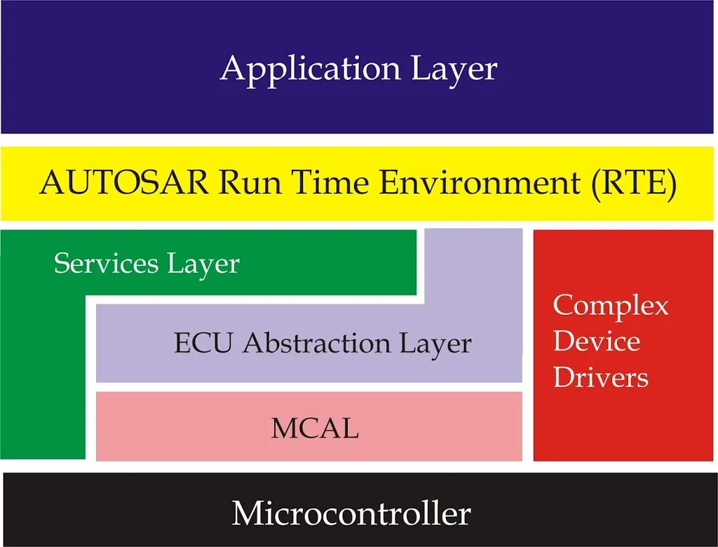
AUTOSAR Architecture
Application Layer: This layer has the application code which resides in top. It can have different application blocks called as Software Components(SWCs) for each feature which the ECU needs to support according to application. For example, the functions like power window and temperature measurement will have separate SWC. This is not a norm, but it depends on the Designer.
AUTOSAR Classic SWC generates ARXML descriptions and algorithmic C code for testing and integration into AUTOSAR RTE.
The AUTOSAR application layer consists of three components which are: application software components, ports of software components, and port interfaces.
Runtime Environment (RTE) provides communication between application software and base software (BSW). The SWC communicates with other components and his BSW module exclusively via his RTE. This allows the SWC to be independent of specific ECUs and other SWCs.
RTE Layer provides ECU independent interfaces to the application software components. The application layer consists of many SWC which does not follow layered architecture style but component style. The Software Components communicate with other components (inter and/or intra ECU) via the RTE.
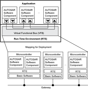
The Classic Platform uses the Virtual Function Bus (VFB) to support hardware-independent development and use of AUTOSAR application software. This bus consists of an abstract representation of the RTE for a specific ECU and separates his AUTOSAR software components of the application layer of the architecture from the architecture infrastructure. AUTOSAR software components and buses communicate using dedicated ports. Configure the application by mapping the ports of the components to the RTE representation of the system ECU.
BSW provides services such as ECU abstraction, microcontroller abstraction, and memory and diagnostics.
Basic Software
Vehicles are equipped with numerous cameras and other sensors both inside and outside them. These sensors are in place to assist the driver in driving, they are used for human vision or machine vision. With a fixed number of sensors already in place, there is a need to utilize them for both machine vision as well as human vision, this gives the need for dedicated algorithms that work with the raw data from the camera making them suitable for the application. Basic software layer is further classified into:
Services Layer,
ECU Abstraction Layer,
Microcontroller Abstraction and Complex Device Drivers (CDD).
Microcontroller Abstraction Layer (MCAL)
The Microcontroller Abstraction Layer is the lowest layer of the Basic Software, this means that MCAL modules can directly access the HW resources. MCAL contains internal drivers which are software modules that are direct access to the µC and internal peripherals.
As the name resembles, the MCAL layer makes the upper layers independent of HW (MCU).
ECU Abstraction Layer
The ECU Abstraction Layer interfaces the drivers of the Microcontroller Abstraction Layer (MCAL). It also contains drivers for external devices within the ECU and provides an abstraction for various peripheral hardware.
It provides interfaces to access all features of an ECU like communication, memory, or I/O, no matter if these features are part of the microcontroller or served by peripheral components.
Complex Device Drivers Layer
The Complex Device Drivers (CDD) Layer spans from the hardware layer to the RTE. CDD fulfills special functions and timing requirements needed to operate complex sensors and actuators.
Provide the possibility to integrate special-purpose functionality. This layer consists of drivers for devices that are not specified within AUTOSAR, with very high timing constrains.
Services Layer
The Services Layer is the topmost layer of the Basic Software (BSW) which also applies its relevance for the application software. It provides an independent Interface of a microcontroller (MCU) and ECU hardware to application software.
The Services Layer offers:
Operating system functionality
Vehicle network communication and management services
Memory services (NVRAM management)
Diagnostic Services (UDS, Error handling, Memory)
ECU state management, mode management
Logical and temporal program flow monitoring (Wdg manager) Task Provide basic services for applications, RTE, and basic software modules.
Advantage of AUTOSAR
AUTOSAR uses a layered architecture which has different layers dedicated to perform different operations and abstraction. The application code is fully portable as AUTOSAR is designed in such a way that the application code is written independent of the hardware so the same application code can run on different hardware platforms. AUTOSAR has a layer dedicated to support hardware functionalities called MCAL (Micro controller abstraction) layer which has drivers for accessing the underlying hardware peripherals of MCU. As AUTOSAR provides standard way of communication, ECUs can communicate with each other irrespective of ECU developer (whether OEM or Tier1) and hence there is no need to maintain custom standard of communication. ECUs utilizing AUTOSAR can communicate with each other irrespective of underlying differences in hardware. Mostly chip manufacturers provides MCAL layer of AUTOSAR, but if they don’t then the developer needs to write his own MCAL layer or outsource to companies providing such services.
Adaptive Platform
Adaptive Platform is distributed computing and service-oriented architecture (SOA). The platform provides high-performance computing, message-based communication mechanisms, and flexible software configurations to support applications such as autonomous driving and infotainment systems. Software based on this platform allows you to:
Meet strict integrity and security requirements
Addresses environmental awareness and motion response planning
Integrate the vehicle into an external system back end or infrastructure
Compatible with external system changes (as software changes are possible during the vehicle’s lifetime)
The RTE layer of the software architecture includes the C++ Standard Library. It supports communication between AUTOSAR software components of the application layer and between AUTOSAR software components and the software provided by the base software layer. The base software layer consists of the system’s underlying software and services. The AUTOSAR software components of the application layer communicate with each other, with services outside the platform, with the underlying software, and with services by responding to event-driven messages. Software components use C++ application programming interfaces (APIs) to interact with software in the base software layer.
The underlying software includes the POSIX operating system and software for system administration tasks, including:
execution management
communication management
time synchronization
identity access management
Logging and tracking
Examples of services include:
Update and configuration management
diagnosis
Signal to service mapping
network management
The ECU hardware on which a single instance of an Adaptive Platform application runs is a machine . A machine can be one or more chips or virtual hardware components. The hardware can be a single chip hosting one or more machines, or multiple chips hosting a single machine.
The Adaptive Platform supports the development and use of hardware-independent AUTOSAR application software. The abstract representation of RTE for a specific ECU (microcontroller, high-performance microcontroller, virtual machine) separates the AUTOSAR software components of the application layer of the architecture from the architectural infrastructure. AUTOSAR software components and underlying software and services communicate using dedicated ports. Configure the application by mapping the ports of the components to the RTE representation of the system ECU.
Comparison between AUTOSAR Classic Platform and Adaptive Platform
purpose or function
Classic Platform
Adaptive Platform
Use Case
embedded system
High-performance computation, communication with external resources, and flexible deployment
programming language
C
C++
operating system
bare board
POSIX
real-time requirements
hard
soft
calculation ability
low
high
communication
signal base
event-based, service-oriented
safety and security
Support available
Support available
dynamic update
It can not be used
Incremental deployment and runtime configuration changes
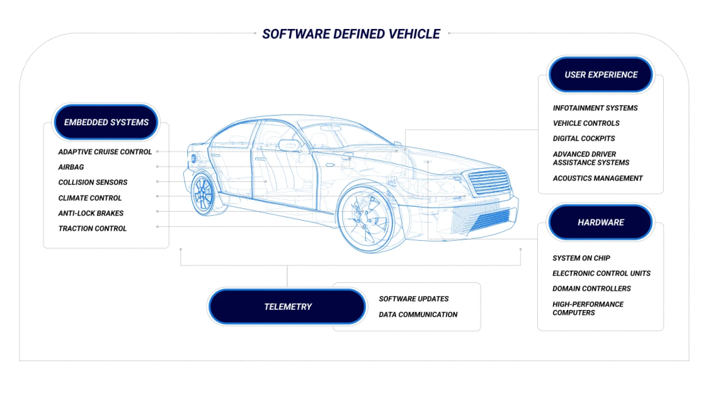
A Software-Defined Vehicle is any vehicle that manages its operations, adds functionality, and enables new features primarily or entirely through software.
it reflects the gradual transformation of automobiles from highly electromechanical terminals to intelligent, expandable mobile electronic terminals that can be continuously upgraded.
To become such intelligent terminals, vehicles are pre-embedded with advanced hardware before standard operating procedures (SOP)—the functions and value of the hardware will be gradually activated and enhanced via the OTA systems throughout the life cycle.
Driving Forces of Software-Defined Vehicles
In the past, the automotive industry stood as a testament to the power of combustion engines and the prestige of owning a car with the “most exhaust pipes.” Today, this old-school paradigm is under‐going a seismic transformation. Four major innovations—electrification, automation, shared mobility, and connected mobility—are happening all at once, leading to dramatic changes in the auto mobile landscape.
Firstly, industry development requirements: software & algorithm— indispensable for the development of connected, autonomous, shared, and electrified automotive technologies.
Secondly, consumers expect similar behaviors and experience from vehicles as with smartphones. Many are left wondering: why can’t my $50,000 car perform the same tasks as my $300 smartphone?
From this frustration emerged the idea of a software-defined vehicle (SDV), a car that’s fully programmable. New features can be developed and deployed within a matter of months, not years, and there’s extra computational capacity for future updates that can be delivered wirelessly.
Goal’s of SDV
it’s about the customer experiences we build. And these customer experiences cannot aim simply to rebuild the smartphone experience.
This is about creating a “habitat on wheels” powered by cross-domain applications and data fusion
Habitat on Wheels
During the past decade, many car manufacturers have sought to replicate successful smartphone applications in their cars. In many cases, however, these in-vehicle applications could not match the quality of the smartphone apps. In addition, consumers usually don’t want redundant experiences, inconsistencies between their digital ecosystems, or the irritation of cumbersome data synchronization.
SDV surpass the concept of a “smartphone on wheels.” Instead, it has to enable a “habitat on wheels,” utilizing the specifics of the car to provide multisensory experiences that a smartphone could never match. With multiple displays and a network of hundreds of sensors and actuators, the SDV brings together domains like infotainment, autonomous driving, intelligent body, cabin and comfort, energy, and connected car services,
Passengers feel recognized as they enter a vehicle personalized to their needs, one that is a clear departure from the impersonal con‐ fines of traditional cars.
SDVs have revolutionized our perception of mobility. It’s no longer merely about getting from point A to point B but about making the journey itself enriching. Thanks to advanced driver-assistance systems and autonomous driving, we’re embracing the transformative, multisensory power of the SDV.
Benefits of Software-Defined Vehicles
The benefits of Software-Defined Vehicles include:
Increased comfort through onboard infotainment systems that integrate connected features such as music and video streaming
Deeper insights into vehicle performance through telematics and diagnostics, allowing for more effective preventative maintenance
The capacity for automotive manufacturers to add new features and functionality with over-the-air updates
Increased value of the vehicle over time as new features are added via software updates
Connectivity between vehicle and smartphone, allowing drivers and passengers to interact with their cars in new ways
Continuous connectivity, delivering real-time information services to and from the vehicle
Cross-Domain Applications and Data Fusion
Today, vehicle experiences often occur in isolated domains. But the future with SDVs promises to blur the boundary between the vehicle and the outside world. Experiences will be cross-domain, where various vehicle functions and systems intercommunicate and interact harmoniously to enrich the overall journey.
Consider the example of a digital “dog mode” that some cars already feature. The vehicle monitors your dog in the car while you are out shopping. Because it is hard for dogs to cool down, a hot car interior on a summer’s day is often enough to cause serious injuries or even death. This is a perfect illustration of customer-centric and cross-domain functionality. It involves multiple systems: the car’s air conditioning to maintain a comfortable temperature, the infotainment screen to display a message letting passers-by know not to worry as the dog is safe and comfy, and the battery management system to ensure the car has sufficient energy. All these domains are coordinated in order to ensure the dog’s safety and comfort.
In this connected ecosystem, your car could even become a creative extension of your social media presence. With your permission, it could capture a stunning sunset through its high-quality on-board cameras during a scenic drive and propose a pre-edited post for your approval.
Cross-domain experiences also extend to personal wellness. Imagine that your fitness wearable signals that you’ve had an intense work‐ out. In response, your car sets the cabin temperature to a cooler setting, selects soothing illumination for the ambient lighting, and plays your favorite cool-down playlist. By seamlessly integrating with your digital devices, your car enhances your post-workout recovery and comfort.
Impediments: Why Is Automotive SoftwareDevelopment Different?
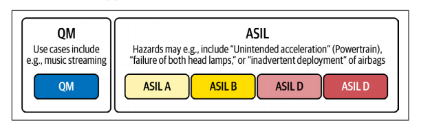
ISO 26262. This standard deals with the functional safety of electrical and electronic systems within vehicles and is fundamental to the concept of an SDV.
To quantify the risk, the standard employs a framework known as Automotive Safety Integrity Levels (ASIL), illustrated in Figure 1-3, which classifies hazardous events that could result from a malfunction based on their level of severity, exposure, and controllability. Levels of risk range from ASIL A, the lowest level, to ASIL D, the highest level. ISO 26262 defines the requirements and safety measures to be applied at each ASIL.
The SDV is more than a simple mobile device; it’s a sophisticated ensemble of systems that prioritizes safety as much as functionality and convenience.
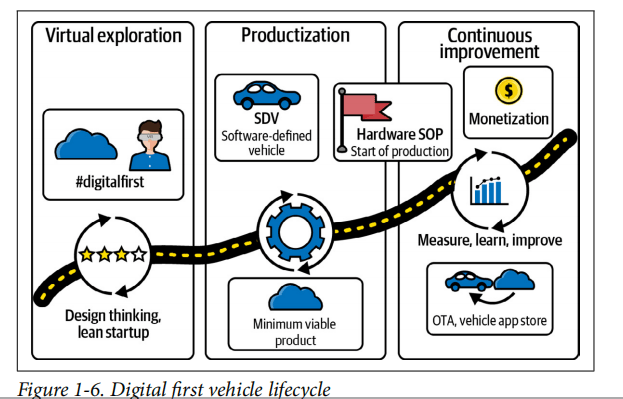
Rethinking the Vehicle Lifecycle: Digital First
Historically, the lifecycle of a vehicle was defined by the simultaneous production and deployment of tightly coupled hardware and software. Once the vehicle was in the consumer’s hands, its features remained essentially unaltered until its end of life. However, an SDV paradigm allows for the decoupling of hardware and software release dates—a prerequisite for a digital first approach, which puts design and virtual validation of the digital vehicle experience at the start of the lifecycle.
Software-Defined Vehicle Architecture
A Software-Defined Vehicle’s software and hardware architecture tend to be incredibly complex, often comprising multiple interconnected software platforms distributed across as many as one hundred electronic control units (ECUs). Some manufacturers are attempting to rationalize this down to fewer ECUs controlled by a very powerful central computer—but either way the architecture of Software-Defined Vehicles can be broken down into four distinctive layers:
1. User Applications
User applications are software and services that interact or interface directly with drivers and passengers. These may include infotainment systems, vehicle controls, digital cockpits, etc.
2. Instrumentation
Systems at the instrumentation layer are generally related to a vehicle’s functionality but don’t typically require direct intervention from a driver. Examples include Advanced Driver Assistance Systems (ADAS) and complex controllers.
3. Embedded OS
The core of the Software-Defined Vehicle, the embedded OS manages everything from sandboxing critical functions to facilitating general operations. These are typically built on microkernel architecture, allowing software capabilities and functionality to be added or removed modularly.
4. Hardware
The hardware layer includes the engine control unit and the chip on which the embedded operating system is installed. All other physical components of the vehicle also fall under this category, including cameras and other vehicle sensors.
Learning from the Smartphone Folks:Standardization, Hardware Abstraction,and App Stores
Today, almost every car model, even those from a single manufacturer, employs custom hardware and software components sourced from various suppliers. The result: extreme fragmentation combined with monolithic programming frameworks, where creating a “vehicle app” that can run across multiple models of the same manufacturer seems nearly impossible. blueprint for overcoming this fragmentation. Its solution was multipronged
A set of standardized vehicle APIs would greatly simplify the process of creating software for vehicles. By ensuring that these APIs have minimal fragmentation, developers could write software once and have it work across multiple vehicle models.
Hardware abstraction layer (HAL). This acts as a bridge between the software applications and the multitude of vehicle hardware variations. It ensures that software can run irrespective of the underlying hardware differences, adding a layer of consistency and predictability.
Supportive software stack (vehicle OS)
A robust software stack that’s in harmony with the standardized APIs and HAL ensures
that software can interact seamlessly with a vehicle’s components, making software-driven innovations easier to introduce and adopt
Vehicle OS and EnablingTechnologies
We will start by looking at emerging electrical and electronic (E/E) architecture Key elements of E/E and SOA are hardware abstraction, vehicle APIs, and the SDV tech stack. Modern vehicles use OTA updates to support post-SOP updates,
we assess the SDV specifically from the perspective of the E/E architecture. We identify the influence of the SDV paradigm on the different functional domains and determine the relevant drivers that must be considered when changing existing solutions. Tapping into our experience as a comprehensive solution provider, we explore how existing archi tecture components such as control units, sensors, actuators, and the wiring harness need to be modernized or replaced and where new solutions need to be added
What is E/E architecture?
In the term “E/E architecture”, E/E stands for “electrical/electronic”, and architecture means “configuration, design concept, and design method”. Combined, E/E architecture is defined as the system that connects in-vehicle ECUs, sensors, actuators, etc.
In recent years, automobiles have evolved rapidly, and they continue to be equipped with new functions, such as driver assistance and automated driving, and functions for connectivity, personalization, and infotainment.
Due to the need for processing that is tailored to each purpose, the number of ECUs installed in automobiles has exceeded one hundred. Innovations in E/E architecture are beginning to be introduced, in order to develop software that simplifies the connection of these increasingly complex ECUs and keeps them in optimal condition.
A brief explanation of domain architecture
Domain architecture classifies ECUs into domains based on their functionality. In contrast, zonal architecture is a new approach that categorizes ECUs based on their physical location within the vehicle and leverages a centralized gateway to manage communication. This physical proximity reduces cabling between ECUs, saving space and reducing vehicle weight, while also improving processor speed.
To understand domain architecture, start with the idea that ECUs are generally divided into five types based on functionality, as shown in Table 1.
Domain
ECU functions
Powertrain domain
Manage vehicle driving functions, including electronic motor control, battery management, engine control, transmission and steering control
Advanced driver assistance systems (ADAS) domain
Processes information from a variety of sensors, including camera modules, radar modules, ultrasound modules, and sensor fusion, and makes decisions to assist the driver
Infotainment domain
Manages in-car entertainment and exchanges information between the car and the outside world, including the head unit, digital cockpit, and telematics control module
Body Electronics/Writing Domain
Manages interior comfort, convenience, and lighting functions, including body control modules, door modules, and headlight control modules
Passive safety domain
Controls safety-related functions such as airbag control module, brake control module, and chassis control module
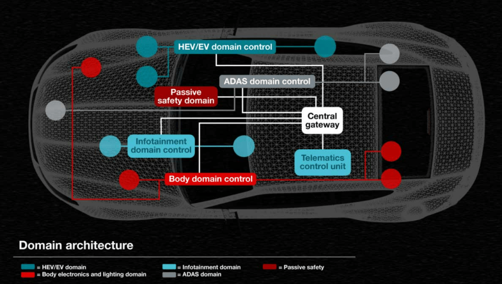
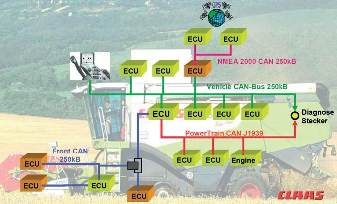
Various ECUs communicate and exchange data via the network. The network is unique and appropriate within each domain, and at the same time communicates with ECUs belonging to external domains. Gateways act as bridges to accommodate the fact that networks in one domain can be different from networks in other domains.
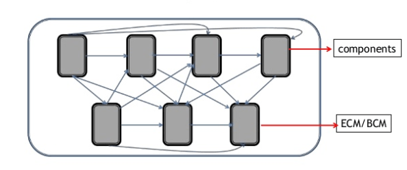
Figure 1 shows a car with a domain-based architecture. In this diagram, one centralized gateway module is connected to various domains within the vehicle. Each domain performs multiple functions. A domain controller, for example a control unit in a car that is responsible for the powertrain, has gateway functionality. This domain gateway supports data communication between the multiple ECUs that make up the domain, and from the domain to other domains within the vehicle.
Zone architecture overview
If we assume that the car is a room and the ECU is a group of people gathered in that room to discuss various topics, then the domain architecture arranges those participants in a chaotic manner. It will be. As a result, each participant must shout loudly (using long cable runs and commensurate power) to be heard by other participants in the conversation group spread across the room.
The car shown in Figure 2 uses a zonal architecture to organize ECUs and add on-board computing modules based on their location in the car. This in-vehicle computing module is a computer with high processing power that can perform all calculations regardless of function. The diagram also shows multiple zone modules and multiple edge nodes associated with each. These exist in different areas of the car.
It is also possible to use a low-bandwidth network, such as a controller area network (CAN), to communicate between the various zone modules and a centralized gateway or computing module. However, a high-speed network like Ethernet is also a good choice. This is because they can provide highly reliable and smooth operation over a wide automotive temperature range. PCIe is a good choice for networks to implement distributed computing between centralized computing modules and zoned modules.
Advantages of zone architecture for power distribution
Engineers can also take advantage of this technique of ECU reorganization to optimize power distribution architectures. In particular, it will be possible to redesign the smart junction box that distributes power to the various loads and ECUs in the car. Specifically, relays and fuses can be replaced with semiconductor solutions.
In a zoned architecture, multiple power distribution boxes are distributed so that each power distribution box can power the modules within its zone. Figure 2 shows the concept of power distribution in a zoned architecture. From this diagram, you can see that each zone’s power distribution function also integrates a zone module that manages network traffic. This new power distribution architecture reduces harness and cable weight. The result is improved fuel efficiency for cars with conventional internal combustion engines, and longer range for electric cars with batteries.
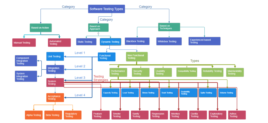
Software testing plays a vital role in ensuring the quality, reliability, and performance of software applications. It covers a diverse range of testing types, each designed to address specific aspects of a software system.
Based on actions:
a. Manual Testing: Manual testing is the process of executing test cases and scenarios without the assistance of automated testing tools. It involves human interaction with the software to ensure its functionality, usability, and to identify any defects or issues.
b. Automated Testing: Automated testing involves the use of scripts or tools to execute and validate predefined test cases, replicating human testing steps. It enables the automatic identification and reporting of bugs or issues in the software, enhancing efficiency and accuracy in the testing process.
Based on Approach:
a. Static Testing: Static testing is a software testing technique that involves reviewing and evaluating the software documentation, code, or other project artifacts without executing the code. Its primary goal is to identify defects, issues, or discrepancies early in the development process, ensuring higher quality by addressing problems at their source.
b. Dynamic Testing: Dynamic testing is a software testing technique that involves the execution of the code to validate its functional behavior and performance. It includes running test cases against the software to assess its functionality, identify defects, and ensure that it meets specified requirements.
Dynamic Testing has 2 types:
1.Functional Testing: Functional testing is a software testing type that verifies that the application’s functions work as intended. It involves testing the software’s features, user interfaces, APIs, databases, and other components to ensure they meet the specified requirements and perform their functions correctly.
2. Non-Functional Testing: Non-functional testing is a type of software testing that assesses aspects of a system that are not related to specific behaviors or functions. It focuses on qualities such as performance, scalability, reliability, usability, and security, ensuring that the software meets requirements related to these non-functional aspects.
Functional Testing has 4 levels:
1.Unit Testing: Unit testing is a software testing technique in which individual units or components of a software application are tested in isolation. The purpose is to validate that each unit functions as designed by checking its coding logic and behavior, typically through automated tests.
2. Integration Testing
a. Component integration testing: Component integration testing checks that different parts of a software system, called components, work well together. It ensures that data is exchanged correctly between these components before moving to more comprehensive testing.
b. System integration testing: System integration testing, in the context of different systems, involves validating the proper flow of data between integrated systems. This testing phase ensures that data exchange and communication between distinct systems occur accurately and according to specified requirements.
System Testing: System testing is a phase of software testing where the entire integrated software system is tested to ensure that it meets the specified requirements. The goal of system testing is to assess the system’s functionality, performance, reliability, and other attributes in a comprehensive manner.
a. Feature testing: Feature testing is a software testing process that specifically focuses on verifying the functionality and behavior of individual features or functionalities within a software application. It aims to ensure that each feature works as intended, meeting the specified requirements, and providing the expected outcomes.
b. Smoke testing: A smoke test is an initial, basic test performed on a software build to check if the essential functionalities of the application work as expected. It aims to identify critical issues early in the testing process, often ensuring that the software build is stable enough for more in-depth testing.
c. Sanity testing: Sanity testing is a brief and focused check performed on related modules of a software application to ensure that recent changes or fixes haven’t adversely affected specific functionalities. It helps quickly verify the stability of the software in key areas after modifications.
d. Regression testing: Regression testing is a type of software testing that verifies whether recent changes to the code, such as new features or bug fixes, have adversely affected the existing functionalities of the software. It involves re-executing previously executed test cases to ensure that the changes haven’t introduced new defects or caused unexpected issues in other parts of the application.
Ad hoc testing: Ad hoc testing is an informal and unplanned approach to software testing, where testers spontaneously and randomly test the application without following any predefined test cases or scripts. The goal is to explore the software in a free-form manner, trying different inputs and interactions to identify unexpected issues or defects. Ad hoc testing is often unstructured and relies on the tester’s experience and intuition to uncover potential problems.
Acceptance Testing: Acceptance testing is a type of software testing that verifies whether a system meets the specified requirements and is acceptable to end-users or stakeholders.
a. Alpha testing: Alpha testing is the initial phase of software testing conducted by the internal development team. It aims to identify and fix issues before releasing the software to a larger audience or to beta testers
b. Beta testing: Beta testing is a phase of software testing where a pre-release version of the software is made available to a selected group of users or the public. The purpose is to gather feedback from real users and identify potential issues or areas for improvement before the official release.
c. Regulatory testing: Regulatory testing refers to the process of testing software applications to ensure compliance with industry regulations, standards, or legal requirements. This type of testing is crucial in sectors where adherence to specific rules and regulations is mandatory, such as finance, healthcare, or government.
What Is Sanity Testing
To understand sanity testing, let’s first understand software build. A software project usually consists of thousands of source code files. It is a complicated and time-consuming task to create an executable program from these source code files. The process to create an executable program uses “build” software and is called “Software Build”.
Sanity testing is performed to check if new module additions to an existing software build are working as expected and can pass to the next level of testing. It is a subset of regression testing and evaluates the quality of regressions made to the software.
Suppose there are minor changes to be made to the code, the sanity test further checks if the end-to-end testing of the build can be performed seamlessly. However, if the test fails, the testing team rejects the software build, thereby saving both time and money.
During this testing, the primary focus is on validating the functionality of the application rather than performing detailed testing. When sanity testing is done for a module or functionality or complete system, the test cases for execution are so selected that they will touch only the important bits and pieces. Thus, it is wide but shallow testing.
What Is Smoke Testing
Smoke Testing is carried out post software build in the early stages of SDLC (software development life cycle) to reveal failures, if any, in the pre-released version of a software. The testing ensures that all core functionalities of the program are working smoothly and cohesively. A similar test is performed on hardware devices to ensure they don’t release smoke when induced with a power supply. Thus, the test gets its name ‘smoke test’. It is a subset of acceptance testing and is normally used in tester acceptance testing, system testing, and integration testing.
The intent of smoke testing is not exhaustive testing but to eliminate errors in the core of the software. It detects errors in the preliminary stage so that no futile efforts are made in the later phases of the SDLC. The main benefit of smoke testing is that integration issues and other errors are detected, and insights are provided at an early stage, thus saving time.
For instance, a smoke test may answer basic questions like “does the program run?”, does the user interface open?”. If this fails, then there’s no point in performing other tests. The team won’t waste further time installing or testing. Thus, smoke tests broadly cover product features within a limited time. They run quickly and provide faster feedback rather than running more extensive test suites that would naturally require much more time.
Sanity Testing vs. Smoke Testing
Smoke testing
Sanity testing
Executed on initial/unstable builds
Performed on stable builds
Verifies the very basic features
Verifies that the bugs have been fixed in the received build and no further issues are introduced
Verify if the software works at all
Verify several specific modules, or the modules impacted by code change
Can be carried out by both testers and developers
Carried out by testers
A subset of acceptance testing
A subset of regression testing
Done when there is a new build
Done after several changes have been made to the previous build
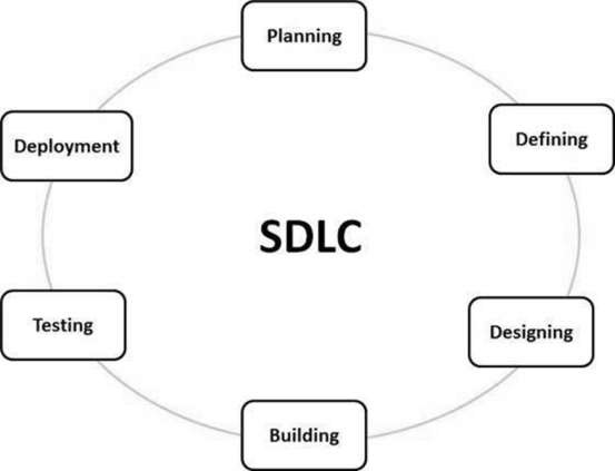
What is the software development life cycle (SDLC)?
Software development is an iterative process that is followed for a software project that consists of several phases for building and running software applications. SDLC helps with the measurement and improvement of a process, which allows an analysis of software development each step of the way.
Why is the SDLC important?
It provides a standardized framework that defines activities and deliverables
It aids in project planning, estimating, and scheduling
It makes project tracking and control easier
It increases visibility on all aspects of the life cycle to all stakeholders involved in the development process
It increases the speed of development
It improves client relations
It decreases project risks
It decreases project management expenses and the overall cost of production
How does the SDLC work?
Stage 1: Planning and Requirement Analysis
Requirement analysis is the most important and fundamental stage in SDLC. It is performed by the senior members of the team with inputs from the customer, the sales department, market surveys and domain experts in the industry. This information is then used to plan the basic project approach and to conduct product feasibility study in the economical, operational and technical areas.
Planning for the quality assurance requirements and identification of the risks associated with the project is also done in the planning stage.
Stage 2: Defining Requirements.
Once the requirement analysis is done the next step is to clearly define and document the product requirements and get them approved from the customer or the market analysts. This is done through an SRS (Software Requirement Specification) document which consists of all the product requirements to be designed and developed during the project life cycle.
Stage 3: Designing the Product Architecture
SRS is the reference for product architects to come out with the best architecture for the product to be developed. Based on the requirements specified in SRS, usually more than one design approach for the product architecture is proposed and documented in a DDS – Design Document Specification.
This DDS is reviewed by all the important stakeholders and based on various parameters as risk assessment, product robustness, design modularity, budget and time constraints, the best design approach is selected for the product.
Stage 4: Building or Developing the Product
In this stage of SDLC the actual development starts and the product is built. The programming code is generated as per DDS during this stage. If the design is performed in a detailed and organized manner, code generation can be accomplished without much hassle.
Stage 5: Testing the Product.
This stage is usually a subset of all the stages as in the modern SDLC models, the testing activities are mostly involved in all the stages of SDLC. However, this stage refers to the testing only stage of the product where product defects are reported, tracked, fixed and retested, until the product reaches the quality standards defined in the SRS.
Stage 6: Deployment in the Market and Maintenance.
Once the product is tested and ready to be deployed it is released formally in the appropriate market. Sometimes product deployment happens in stages as per the business strategy of that organization. The product may first be released in a limited segment and tested in the real business environment (UAT- User acceptance testing).
SDLC Models
There are various software development life cycle models defined and designed which are followed during the software development process. These models are also referred as Software Development Process Models”. Each process model follows a Series of steps unique to its type to ensure success in the process of software development
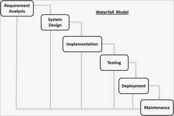
Waterfall Model
This SDLC model is the oldest and most straightforward. With this methodology, we finish one phase and then start the next. Each phase has its own mini-plan and each phase “waterfalls” into the next. The biggest drawback of this model is that small details left incomplete can hold up the entire process.
The next phase is started only after the defined set of goals are achieved for previous phase and it is signed off, so the name “Waterfall Model”. In this model, phases do not overlap.
Some situations where the use of Waterfall model is most appropriate are −
Requirements are very well documented, clear and fixed.
Product definition is stable.
Technology is understood and is not dynamic.
There are no ambiguous requirements.
Ample resources with required expertise are available to support the product.
The project is short
Some of the major advantages of the Waterfall Model are as follows −
Simple and easy to understand and use
Easy to manage due to the rigidity of the model. Each phase has specific deliverables and a review process.
Phases are processed and completed one at a time.
Works well for smaller projects where requirements are very well understood.
Clearly defined stages.
Well understood milestones.
Easy to arrange tasks.
Process and results are well documented.
Waterfall Model – Disadvantages
The disadvantage of waterfall development is that it does not allow much reflection or revision. Once an application is in the testing stage, it is very difficult to go back and change something that was not well-documented or thought upon in the concept stage.
The major disadvantages of the Waterfall Model are as follows −
No working software is produced until late during the life cycle.
High amounts of risk and uncertainty.
Not a good model for complex and object-oriented projects.
Poor model for long and ongoing projects.
Not suitable for the projects where requirements are at a moderate to high risk of changing. So, risk and uncertainty is high with this process model.
It is difficult to measure progress within stages.
Cannot accommodate changing requirements.
Adjusting scope during the life cycle can end a project.
Integration is done as a “big-bang. at the very end, which doesn’t allow identifying any technological or business bottleneck or challenges early.
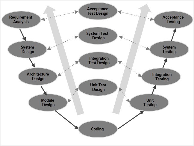
V-Model – Design
The V-model is an SDLC model where execution of processes happens in a sequential manner in a V-shape. It is also known as Verification and Validation model.
The V-Model is an extension of the waterfall model and is based on the association of a testing phase for each corresponding development stage.
This means that for every single phase in the development cycle, there is a directly associated testing phase. This is a highly-disciplined model and the next phase starts only after completion of the previous phase
SDLC – Agile Model
Agile SDLC model is a combination of iterative and incremental process models with focus on process adaptability and customer satisfaction by rapid delivery of working software product. Agile Methods break the product into small incremental builds. These builds are provided in iterations. Each iteration typically lasts from about one to three weeks.
Agile planning is an iterative approach to managing projects avoiding the traditional concept of detailed project planning with a fixed date and scope.
Agile project planning emphasizes frequent value delivery, constant end-user feedback, cross-functional collaboration, and continuous improvement.
Unlike traditional project planning, Agile planning remains flexible and adaptable to changes that may emerge at any project lifecycle stage.
Following are the Agile Manifesto principles −
Individuals and interactions − In Agile development, self-organization and motivation are important, as are interactions like co-location and pair programming.
Working software − Demo working software is considered the best means of communication with the customers to understand their requirements, instead of just depending on documentation.
Customer collaboration − As the requirements cannot be gathered completely in the beginning of the project due to various factors, continuous customer interaction is very important to get proper product requirements.
Responding to change − Agile Development is focused on quick responses to change and continuous development.
What Are the Steps in the Agile Planning Process?
Define project goals: project planning starts with clearly defining what the purpose of this project is. This will create direction for the team to follow and ensure that all efforts are aligned with the primary goals.
Load backlog with work items: identify what needs to be done to complete a project. Agile teams use work elements like initiatives, epics/ projects and tasks/ user stories to build their work structure and create an alignment between the project goals and execution.
Release planning: review the backlog and determine the order of work execution. In Scrum, teams conduct Sprint planning, choosing the next highest priority items to execute in the sprint. Kanban teams use historical data to estimate project length and use Kanban boards as a planning tool to prioritize upcoming work.
Daily stand-up: holding a daily meeting will ensure everyone on the team is in the loop. This meeting aims to identify and resolve issues, find new opportunities for improvement and discuss project progress.
Process review: examine the end-to-end flow of work from initiation to customer delivery. Gather feedback to identify areas for future improvements. Scrum teams do that during Sprint Review and Retrospective meetings, while Kanban teams have Service Delivery Review meetings.
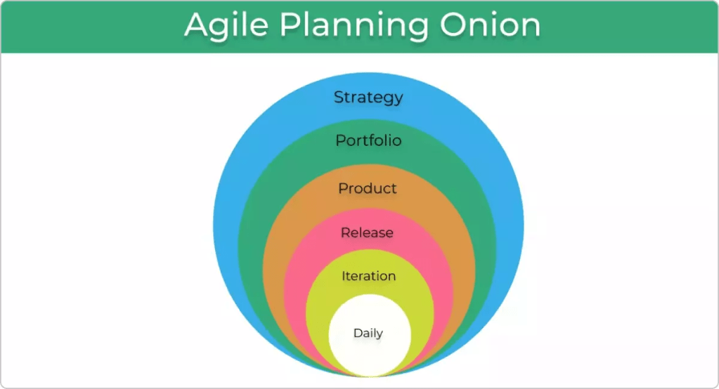
The 6 Levels of Agile Planning
Let’s have a look at each level from a product development perspective:
Strategy: The outermost layer of the onion represents the overall strategic vision and goals of an organization and how they are going to be achieved. It is usually conducted by the senior leadership team.
Portfolio: At this level, senior managers discuss and plan out the portfolio of products and services that will support the execution of the strategy defined in the previous level.
Product: Teams create a high-level plan and break it down into significant deliverables of key features and functionalities that will contribute to accomplishing the strategic objectives.
Release: The key features defined are set to be delivered within a time-framed box (usually a month).
Iteration: This level focuses on managing work in a timeframe of a few weeks. Teams select several individual tasks or user stories from the backlog to deliver in small batches.
Daily: The goal of the daily planning meetings is for teams to walk through their tasks and discuss project progress and any impediments threatening the process. During this time, they create an action plan for the next steps of the project execution.
What Is DevOps?
DevOps is a set of practices, tools, and a cultural philosophy that automate and integrate the processes between software development and IT teams. It emphasizes team empowerment, cross-team communication and collaboration, and technology automation.
The original meaning of the term DevOps is to automate and unify the efforts of two groups, development teams and IT operations teams, that have traditionally operated separately, charting a path for change in software development processes and organizational culture. Delivering high quality software quickly.
DevOps represents the current state of evolution of the software delivery cycle over the past 20 years. This ranges from huge code releases of entire applications every few months or years to iterative updates of small features and functionality released daily or several times a day.
DevOps integrates and automates the work of software development and IT operations teams, enabling them to deliver high-quality software quickly.
In reality, a very good DevOps process and culture extends beyond development and operations and includes all application stakeholders (platform and infrastructure engineering, security, compliance, governance, risk management, line-of-business, , end users, and customers) into the software development lifecycle.
DevOps represents the current state of evolution of the software delivery cycle over the past 20 years. This ranges from huge code releases of entire applications every few months or years to iterative updates of small features and functionality released daily or several times a day.
Ultimately, DevOps is about meeting the ever-increasing demands of software users for frequently released innovative new features and uninterrupted performance and availability.
How DevOps was born?
Just before the year 2000, most software was developed and updated using a waterfall methodology, a linear approach to large-scale development projects. The software development team had spent months developing a huge body of new code. This code affected most or all of the application, and the changes were so extensive that the development team spent several additional months integrating the new code into the code base.
Quality assurance (QA), security, and operations teams then spent several more months testing the code. As a result, software releases range from months to years, often with several important patches and bug fixes between releases. This big bang approach to feature delivery has three characteristics.
To speed development and improve quality, the development team began adopting agile software development methodologies. This approach is iterative rather than linear and emphasizes making smaller, more frequent updates to the application’s code base. At the heart of these methods are continuous integration and continuous delivery , or CI/CD. Small chunks of new code from CI/CD are merged into the code base every week or two, then automatically integrated, tested, and ready to be deployed to production
The more effectively these agile development practices accelerate software development and delivery, the more effectively IT operations (system provisioning, configuration, acceptance testing, management, and monitoring), still in silos, become part of the software delivery lifecycle. The next bottleneck became even more obvious.
This is how DevOps was born from agile methods. DevOps has added new processes and tools to extend the continuous iteration and automation of CI/CD to other parts of the software delivery lifecycle. We also ensured close collaboration between development and operations at every stage of the process.
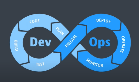
How DevOps works: DevOps lifecycle
Planning (or ideation). In this workflow, the team takes a closer look at the features and functionality that should be included in the next release. This includes prioritized end-user feedback, customer stories, and input from all internal stakeholders. The goal during this planning stage is to maximize the business value of the product by creating a backlog of features that will produce valuable and desired outcomes when delivered.
development. This is the programming phase, where developers test, code, and build new features and enhancements based on user stories and work items in the backlog
Integration (build, or continuous integration and continuous delivery (CI/CD)). As mentioned above, this workflow integrates new code into an existing code base, then tests it, and packages it into an executable file for deployment.
Deployment (usually called continuous deployment ). Here the runtime build output (from the integration) is deployed to a runtime environment (this environment typically refers to a development environment where runtime tests are performed for quality, compliance, and security)
Operation. Manage the end-to-end delivery of IT services to customers. This includes the practices involved in design, implementation, configuration, deployment, and maintenance of all IT infrastructure that supports an organization’s services.
Observe : Quickly identify and resolve issues that impact product uptime, speed, and functionality. Automatically notify your team of changes, high-risk actions, or failures, so you can keep services on.
Continuous feedback
DevOps teams should evaluate each release and generate reports to improve future releases. By gathering continuous feedback, teams can improve their processes and incorporate customer feedback to improve the next release.
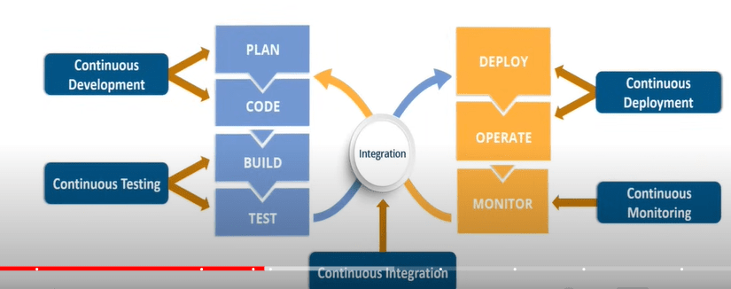
Three other important continuous workflows occur in between these workflows.
Continuous testing: The classic DevOps lifecycle includes a separate “testing” phase that occurs between integration and deployment. However, with evolved DevOps, planning (behavioral-driven development), development (unit testing, contract testing), integration (static code scanning, CVE scanning, linting), and deployment (smoke testing, penetration testing, configuration testing) Certain elements of testing now occur during , production (chaos testing, compliance testing), and learning (A/B testing)
Security: Waterfall methodologies and agile implementations “add” security workflows after delivery or deployment. DevOps, on the other hand, aims to embed security from the beginning (planning), when security issues are easiest and least expensive to resolve, and throughout the remaining stages of the development cycle. This has led to the rise of DevSecOps
Compliance: with laws and regulations Compliance (governance and risk) efforts are also best addressed early and throughout the development lifecycle. Regulated industries are frequently mandated to provide a certain level of observability, traceability, and access to how functionality is delivered and managed in the runtime production environment
DevOps Tools
Project management tools: Tools that allow teams to create a backlog of user stories (requirements) that make up a coding project, break the project into smaller tasks, and track tasks to completion. Many tools support the agile project management methodologies that developers are adopting for DevOps, such as Scrum, Lean, and Kanban. Popular open source options include GitHub Issues and Jira.
Jira Product Discovery organizes this information into actionable inputs and prioritizes actions for development teams.
we recommend tools that allow development and operations teams to break work down into smaller, manageable chunks for quicker deployments. This allows you to learn from users sooner and helps with optimizing a product based on the feedback. Look for tools that provide sprint planning, issue tracking, and allow collaboration, such as Jira.
Build
Collaborative source code repository: A version-controlled coding environment. Multiple developers can work on the same code base. The code repository integrates with CI/CD, testing, and security tools so that when code is committed to the repository, you can automatically take the next step. Open source code repositories include GiHub and GitLab.
A framework within which people can address complex adaptive problems, while productively and creatively delivering products of the highest possible value.”
In simple terms, scrum is a lightweight agile project management framework that can be used to manage iterative and incremental projects of all types. The concept here is to break large complex projects into smaller stages, reviewing and adapting along the way
History of Scrum
The term “scrum” was first introduced by two professors Hirotaka Takeuchi and Ikujiro Nonaka in the year 1986, in Harvard Business Review article. There they described it as a “rugby” style approach to product development, one where a team moves forward while passing a ball back and forth.
Software developers Ken Schwaber and Jeff Sutherland each came up with their own version of Scrum, which they presented at a conference in Austin, Texan in 1995. In the year 2010, the first publication of official scrum guide came out.
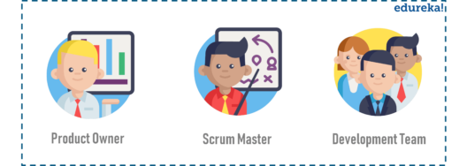
Scrum Roles
There are three distinct roles defined in Scrum:
The Product Owner is responsible for the work the team is supposed to complete. The main role of a product owner is to motivate the team to achieve the goaland the vision of the project. While a project owner can take input from others but when it comes to making major decisions, ultimately he/she is responsible.
The Scrum Master ensures that all the team members follow scrum’s theories, rules, and practices. They make sure the Scrum Team has whatever it needs to complete its work, like removing roadblocks that are holding up progress, organizing meetings, dealing with challenges and bottlenecks
The Development Team(Scrum Team) is a self-organizing and a cross-functional team, working together to deliver products. Scrum development teams are given the freedom to organize themselves and manage their own work to maximize the team’s effectiveness and efficiency.
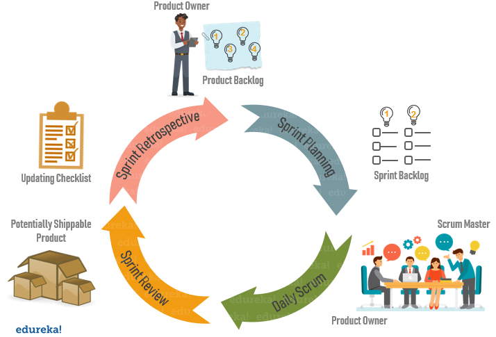
Events in Scrum
In particular, there are four events that you will encounter during the scrum process. But before we proceed any further you should be aware of what sprint is.
A sprint basically is a specified time period during which a scrum team produces a product.
The four events or ceremonies of Scrum Framework are:
Sprint Planning: It is a meeting where the work to be done during a sprint is mapped out and the team members are assigned the work necessary to achieve that goal.
Daily Scrum: Also known as a stand-up, it is a 15-minute daily meeting where the team has a chance to get on the same page and put together a strategy for the next 24 hours.
Sprint Review: During the sprint review, product owner explains what the planned work was and what was not completed during the Sprint. The team then presents completed work and discuss what went well and how problems were solved.
Sprint Retrospective: During sprint retrospective, the team discusses what went right, what went wrong, and how to improve. They decide on how to fix the problems and create a plan for improvements to be enacted during the next sprint.
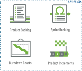
Scrum Artifacts
Artifacts are just physical records that provide project details when developing a product. Scrum Artifacts include:
Product Backlog: It is a simple document that outlines the list of tasks and every requirement that the final product needs. It is constantly evolving and is never complete. For each item in the product backlog, you should add some additional information like:
Description
Order based on priority
Estimate
Value to the business
Sprint Backlog: It is the list of all items from the product backlog that need to be worked on during a sprint. Team members sign up for tasks based on their skills and priorities. It is a real-time picture of the work that the team currently plans to complete during the sprint.
Burndown Chart: It is a graphical representation of the amount of estimated remaining work. Typically the amount of remaining work is will featured on the vertical axis with time along the horizontal axis.
Product Increment: The most important artifact is the product improvement, or in other words, the sum of product work completed during a Sprint, combined with all work completed during previous sprints.
Key Features of Effective Scrum Tools
When assessing Scrum tools, one must consider features like the capability of sprint management, monitoring of tasks, and performance evaluation. Specifically, Scrum tools must include the following features:
The tool must be able to generate a task board offering a visual representation of the progress of ongoing sprints.
They must document user stories. It means an informal explanation of features from the user’s point of view that aids in understanding the goal of the team collectively.
They should have the potential to conduct sprint planning, including defining each sprint concerning the goal, workflow, team assigned, task, and outcome.
They must provide real-time updates. For instance, it tracks the status of the ongoing task in percentages on the task board.
1. Best for backlog management: Jira Software.
2. Best for documentation and knowledge management: Confluence
3. Best for sprint planning: Jira Software
4. Best for sprint retrospective: Confluence whiteboards
Put simply, Agile project management is a project philosophy or framework that takes an iterative approach towards the completion of a project.
There are many different project management methodologies used to implement the Agile philosophy. Some of the most common include Kanban, Extreme Programming (XP), and Scrum.
Scrum project management is one of the most popular Agile methodologies used by project managers.
“Whereas Agile is a philosophy or orientation, Scrum is a specific methodology for how one manages a project,” Griffin says. “It provides a process for how to identify the work, who will do the work, how it will be done, and when it will be completed by.”
Agile is a philosophy, whereas Scrum is a type of Agile methodology
Scrum is broken down into shorter sprints and smaller deliverables, while in Agile everything is delivered at the end of the project
Agile involves members from various cross-functional teams, while a Scrum project team includes specific roles, such as the Scrum Master and Product Owner
WHEN TO USE SCRUM IN YOUR PROJECT
1. WHEN REQUIREMENTS ARE NOT CLEARLY DEFINED
2. WHEN THE PROBABILITY OF CHANGES DURING THE DEVELOPMENT IS HIGH
3. WHEN THERE IS A NEED TO TEST THE SOLUTION
4. WHEN THE PRODUCT OWNER (PO) IS FULLY AVAILABLE
5. WHEN THE TEAM HAS SELF-MANAGEMENT SKILLS
7. WHEN THE CLIENT’S CULTURE IS OPEN TO INNOVATION AND ADAPTS TO CHANGE
The key Scrum advantages
Adaptable and flexible
Adaptation is at the heart of the Scrum framework. It’s suitable for situations where the scope and requirements are not clearly defined. Changes can be quickly integrated into the project without affecting project output.
Faster delivery
Since the goal is to produce a working product with every sprint, Scrum can result in faster delivery and an earlier time to market. In more traditional frameworks, completed work is finished in total at the end of the project.
Encourages creativity
In Scrum, there is a focus on continuous improvement, and Scrum teams embrace new ideas and techniques. This leads to better quality, which allows your products to stand out in an increasingly competitive market.
Lower costs
Scrum can be cost-effective for organizations as it requires less documentation and control. It can also lead to increased productivity for the Scrum team, meaning less time and effort is wasted.
Improves customer satisfaction
Better quality work means greater customer satisfaction. Clients can test the product at the end of each sprint and communicate their feedback to the team. Since Scrum is designed for adaptability, changes can be made quickly and easily.
Improves employee morale
Every member of the Scrum team takes full ownership of their work, with the Scrum master on hand to support and protect them from outside pressure. As a result, team members feel capable and motivated to do their best work.
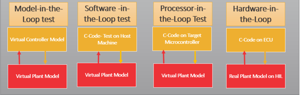
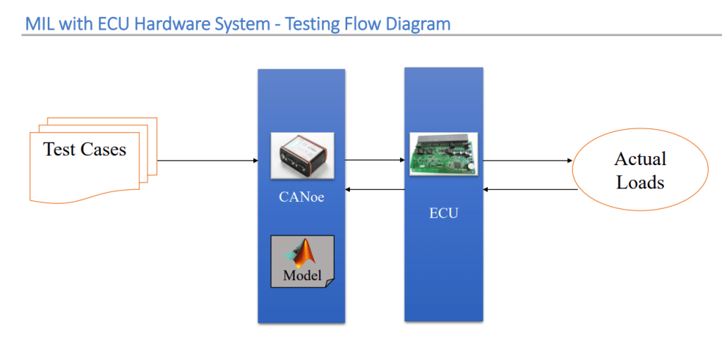
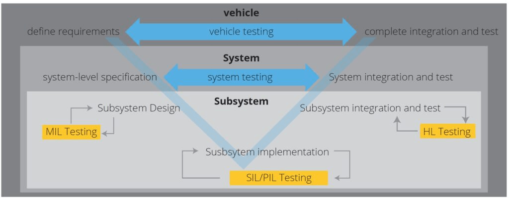
supports requirements development, design, analysis, verification, and validation of complex systems Verification (simulation) and validation (testing) are key elements of MBSE. Model in the loop (MIL), software in the loop (SIL), processor in the loop (PIL), and hardware in the loop (HIL) simulation and testing take place at specific points during the MBSE process to ensure a robust and reliable result.
MIL, SIL, PIL, and HIL testing come in the verification part of the Model-Based Design approach after you have recognized the requirement of the component/system you are developing and they have been modeled at the simulation level (e.g. Simulink platform). Before the model is deployed to the hardware for production, a few verification steps take place which are listed below.
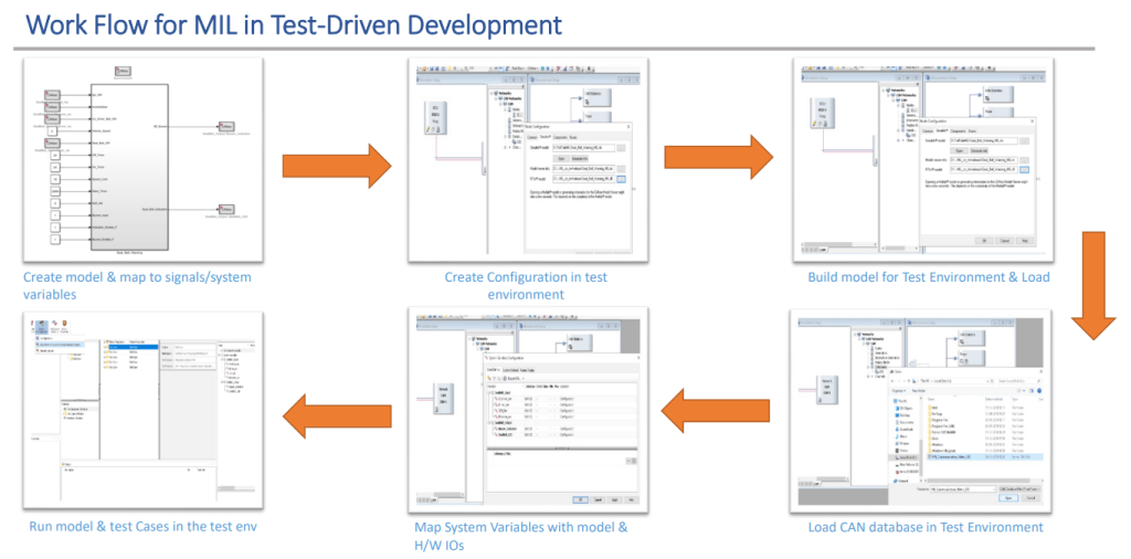
Model-in-the-Loop (MIL) simulation or Model-Based Testing
First, you have to develop a model of the actual plant (hardware) in a simulation environment such as Simulink, which captures most of the important features of the hardware system. After the plant model is created, develop the controller model and verify if the controller can control the plant (which is the model of the motor in this case) as per the requirement. This step is called Model-in-Loop (MIL) and you are testing the controller logic on the simulated model of the plant. If your controller works as desired, you should record the input and output of the controller which will be used in the later stage of verification.
MIL testing is used to evaluate the functionality of a system model in a simulated environment. This is typically done by connecting the model to a simulator that represents the system’s environment.
For example, after a plant model has been developed, MIL is used to validate that the controller module can control the plant as desired. It verifies that the controller logic produces the required functionality.
2) Software-in-the-Loop (SIL) simulation
Once your model has been verified in MIL simulation, the next stage is Software-in-Loop(SIL), where you generate code only from the controller model and replace the controller block with this code. Then run the simulation with the Controller block (which contains the C code) and the Plant, which is still the software model (similar to the first step). This step will give you an idea of whether your control logic i.e., the Controller model can be converted to code and if it is hardware implementable. You should log the input-output here and match it with what you have achieved in the previous step. If you experience a huge difference in them, you may have to go back to MIL and make necessary changes and then repeat steps 1 and 2. If you have a model which has been tested for SIL and the performance is acceptable you can move forward to the next step.
3) Processor-in-the-Loop (PIL) or FPGA-in-the-Loop (FIL) simulation
The next step is Processor-in-the-Loop (PIL) testing. In this step, we will put the Controller model onto an embedded processor and run a closed-loop simulation with the simulated Plant. So, we will replace the Controller Subsystem with a PIL block which will have the Controller code running on the hardware. This step will help you identify if the processor is capable of running the developed Control logic. If there are glitches, then go back to your code, SIL or MIL, and rectify them.
4) Hardware-in-the-Loop (HIL) Simulation
Before connecting the embedded processor to the actual hardware, you can run the simulated plant model on a real-time system such as Speedgoat. The real-time system performs deterministic simulations and have physical real connections to the embedded processor, for example analog inputs and outputs, and communication interfaces such as CAN and UDP. This will help you with identifying issues related to the communication channels and I/O interface, for example, attenuation and delay which are introduced by an analog channel and can make the controller unstable. These behaviors cannot be captured in simulation. HIL testing is typically performed for safety-critical applications, and it is required by automotive and aerospace validation standards
The software development life cycle from the initial definition of requirements to the completed integration process and deployment.
Importance of early and thorough design verification
MBE approaches can provide early design verification and speed the development process. MBSE, for example, is particularly valuable in numerous scenarios such as:
Complex systems. Increasing functional complexity from generation to generation can exponentially complicate the design process, especially when new functionalities are added on top of an existing system, such as vehicles with more and more advanced driver assistance system (ADAS) functions that must work in harmony and share access to multiple electronic control units (ECUs).
Stricter safety and performance requirements. Safety and performance expectations for aerospace systems, vehicles, and even Industry 4.0 cyber-physical systems are increasingly complex. MBSE tools support early-stage testing and simulations that can save time and expense while still meeting challenging performance and safety requirements.
Cost and time to market. Better, faster, cheaper has been the mantra of the electronics industry for decades, and that same expectation now extends to complex systems. The use of MBD and MBSE enables faster development of increasingly complex cyber-physical systems and systems of systems, and that in turn supports better system performance and reduced costs.
This is the first post on my new blog “Automotive Diagnostics“.
Diagnostics , OBD-2 , CAN Protocol , CAN FD , Ethernet , Automotive Ethernet ,OSI Layers, VLAN and DOIP. Some of This very hot Buzz words swirling around . And many of us are confused how to learn and Differentiate Between this terms . Raise Your hand if You are also among them.
Ok Well..Bring down your hand Buddy in this series I will cover All this terms in simpler way from Beginner point of view . Following topics will be covered here in this Blog:
Introduction to Automotive Diagnostics.
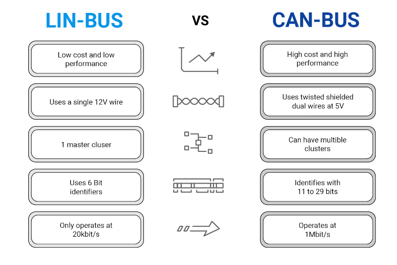
Vehicle Bus System & CAN Protocol Part-1
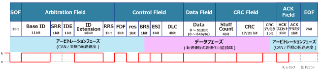
CAN Protocol Part-2
CAN Protocol & CAN FD Part-3
Unified Diagnostic services (UDS)**
Introduction to Ethernet
Automotive Ethernet
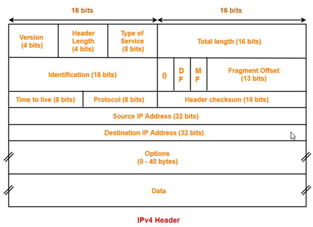
IPv-4 Addressing**
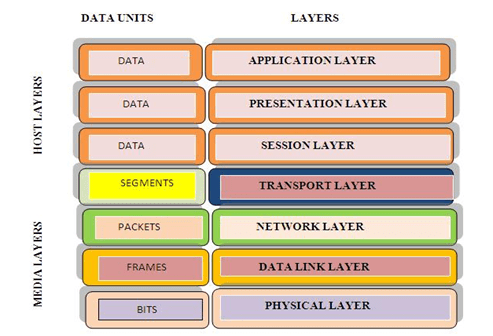
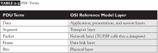
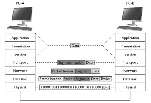
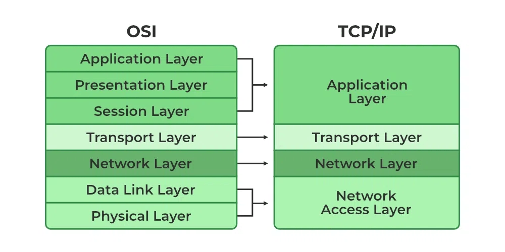
OSI Model and TCP/IP Model
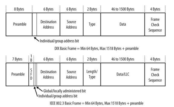
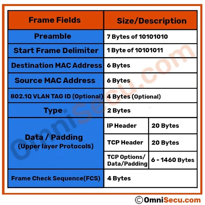
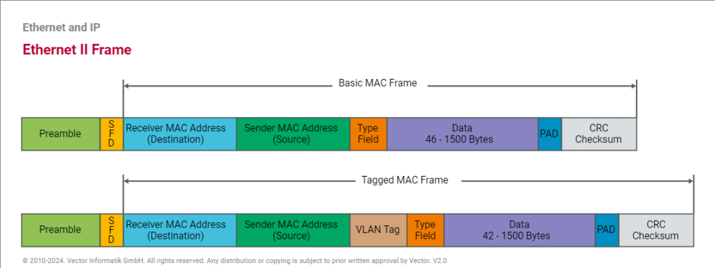
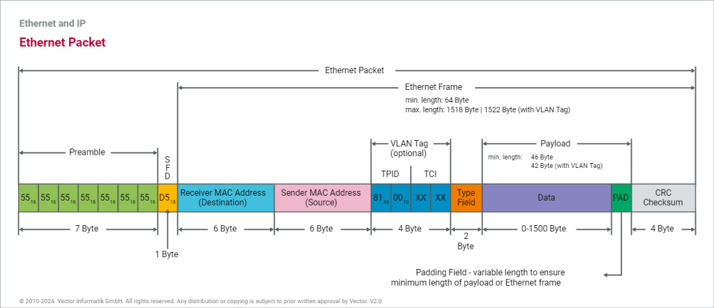
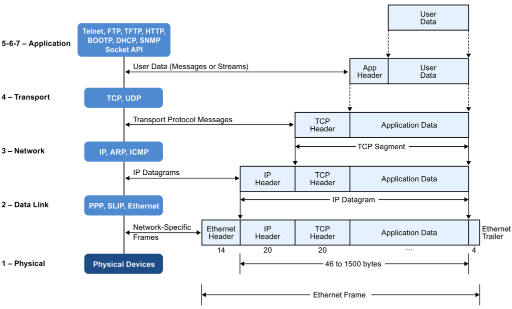
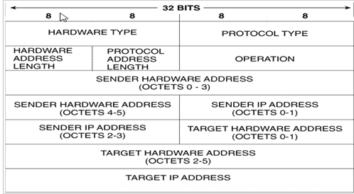
Encapsulation ,DE-Encapsulation & Different Standards Ethernet Frame Format**.
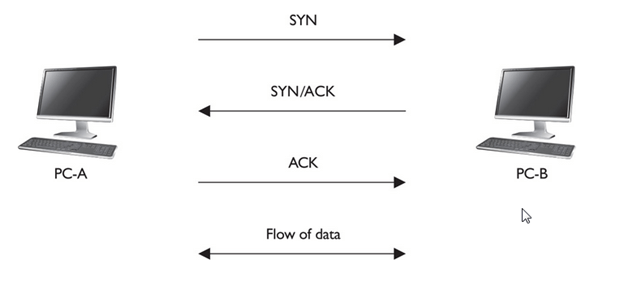
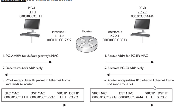
Complete END to END Connection Establishment with Example
Introduction to DOIP & Gateway**
Note: ** Topics are yet to be updated with More detail
All this topic will be covered in Much detail for eg in 100 Base T1 we will cover meaning of each term like what 100 ,Base ,T & 1 stands for and all such minutiae Details will be covered in Each Topic . So Let’s Start The Journey & Happy Learning…..
An automobile as we know it was not invented in a single day by a single inventor. It is more than an engine and a body; it is a complex machine that has undergone over a century of evolution Detecting a failure in this complex machine would be a tedious task. However, most of the vehicles today include computers (Electronic Control Unit (ECU)), which monitors several sensors, located throughout the engine, fuel and exhaust systems. When the computer system of the car detects a fault, two things are supposed to happen/monitored. First, a warning light on the dashboard is set, to inform the driver that a problem exists. Second the code is recorded in the computer’s memory (Electrically Erasable Programmable Read-Only Memory) so that it can later be retrieved by a technician for diagnosis and repair.
When the Check Engine Light comes on, a diagnostic trouble code (DTC) is recorded in the on-board computer memory that corresponds to the fault. Some problems can generate more than one trouble code, and some vehicles may have multiple problems that set multiple trouble codes.
Engine/Electronic Control Unit (ECU)
The ECU can refer to a single module or a collection of modules. These are the brains of the vehicle. They monitor and control many functions of the car. These can be standard from the manufacturer, reprogrammable, or have the capability of being daisy-chained for multiple features. Tuning features on the ECU can allow the user to make the engine function at various performance levels and various economy levels. On new cars, these are all typically microcontrollers.
Some of the more common ECU types include:
• Engine Control Module (ECM) – This controls the actuators of the engine, affecting things like ignition timing, air to fuel ratios, and idle speeds.
• Vehicle Control Module (VCM) – Another module name that controls the engine and vehicle performance.
• Transmission Control Module (TCM) – This handles the transmission, including items like transmission fluid temperature, throttle position, and wheel speed.
• Powertrain Control Module (PCM) – Typically, a combination of an ECM and a TCM. This controls your powertrain.
• Electronic Brake Control Module (EBCM) – This controls and reads data from the anti-lock braking system (ABS).
• Body Control Module (BCM) – The module that controls vehicle body features, such as power windows, power seats, etc.
What is Vehicle Diagnostics ?
Modern vehicles are packed full of modules, all continuously monitoring themselves and reporting their status.
Detecting a failure in this complex machine would be a tedious task. However, most of the vehicles today include computers (Electronic Control Unit (ECU)), which monitors several sensors, located throughout the vehicle.
When the computer system of the car detects a fault, two things are supposed to happen/monitored.
First, a warning light on the dashboard (MIL – Malfunction Indication Light) is set, to inform the driver that a problem exists.
Second the code is recorded in the computer’s memory (EEPROM) so that it can later be retrieved by a technician for diagnosis and repair.
Diagnostics, as the word suggests, is to identify the cause of a problem or a situation. Whenever the ECU finds a problem, it stores that problem as a Diagnostics Trouble Code (DTC) in the ElectricallyErasableProgrammableRead-OnlyMemory (EEPROM) for later retrieval.
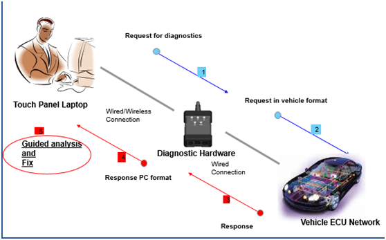
A diagnostic equipment allows you to diagnose and fix the problem with the vehicle. Diagnostic Tools are used to read data (DTC’s) from the EEPROM to analyze the cause of failure.
Such an equipment will communicate with the vehicle and for this, it requires basically a communication medium and a communication protocol
Malfunction Indicator Lamp (MIL)
The MIL is that terrible little light in the dash that indicates a problem with the car. There are a few variations, but they all indicate an error found by the OBD-II protocol.
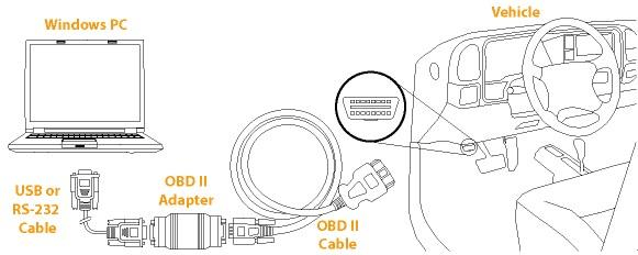
Vehicle Communication Interfaces (VCI)
VCI provide an interface between a vehicle’s onboard diagnostics link (e.g. OBD) and a diagnostic application
▪ Features
▪ Enable communication between offboard device and ECU
via multiple communication protocol
– Supports ECU reprogramming
.
Diagnostics Protocol
Protocol refers to a set of rules for communication. Here the communication happens between two ECU’s which follow the same rule and able to exchange the information. The protocols which are used for Diagnostics purposes are known as Diagnostics Protocol. The automotive industry has come up with Diagnostics protocols which are used for diagnostics purposes like, CAN (Control Area Network), K-Line, UDS (Unified Diagnostics Services), and KWP (Keyword Protocol) and so on.
Diagnostics Session
Diagnostic session is the basis for/of communication between the ECU and the diagnostic tool. During ‘Diagnostics’ the ECU being analyzed is in a particular session. Basically there are different types of diagnostics sessions likeDefault Session, Extended Diagnostic Session and ECU Programming Session. After Ignition on, ECU will be switched to a Default Diagnostic Session and after receiving the request from Diagnostic Tool, the ECU will be switched to the Extended Diagnostic Session. Further, after receiving the ECU Programming Session start request from Diagnostic tool, it will switch to the ECU Programming Session.
Diagnostic Trouble Codes
Diagnostic Trouble Codes or OBD2 Trouble Codes are codes that the
car’s OBD system uses to notify you about an issue. Each code
corresponds to a fault detected in the car. When the vehicle detects an
issue, it will activate the corresponding trouble code.
A vehicle stores the trouble code in it’s memory when it detects a
component or system that’s not operating within acceptable limits. The
code will help you to identify and fix the issue within the car.
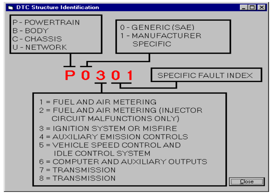
Each trouble code consists of one letter and four digits, such as P1234
Format of the OBD2 Trouble Codes
The OBD2 Trouble Codes are categorized into four different systems.
Body (B-codes) category covers functions that are, generally, inside of the passenger compartment. These functions provide the driver with assistance, comfort, convenience, and safety.
Chassis (C-codes) category covers functions that are, generally, outside of the passenger compartment. These functions typically include mechanical systems such as brakes, steering and suspension.
Powertrain (P-codes) category covers functions that include engine, transmission and associated drive train accessories.
Network & Vehicle Integration (U-codes) category covers functions that are shared among computers and systems on the vehicle.
Generic and manufacturer specific codes
The first digit in the code will tell you if the code is a generic or manufacturer specific code.
Codes starting with 0 as the first digit are generic
or global codes. It means that they are adopted by all cars that follow
the OBD2 standard. These codes are common enough across most
manufacturers so that a common code and fault message could be assigned.
Codes starting with 1 as the first digit are
manufacturer specific or enhanced codes. It means that these codes are
unique to a specific car make or model. These fault codes will not be
used generally by a majority of the manufacturers.
What is OBD?
OBD stands for “On-Board Diagnostics.” It is a computer-based system originally designed to reduce emissions by monitoring the performance of major engine components.
A basic OBD system consists of an ECU (Electronic Control Unit), which uses input from various sensors (e.g., oxygen sensors) to control the actuators (e.g., fuel injectors) to get the desired performance. The “Check Engine” light, also known as the MIL (Malfunction Indicator Light), provides an early warning of malfunctions to the vehicle owner
On-Board Diagnostics (OBD) is your vehicle’s built-in self-diagnostic
system
Indicates when there’s an error via the ‘malfunction indicator light’
Allows a mechanic (or you) to troubleshoot by scanning for Diagnostic Trouble Codes (DTCs)
OBD2 runs on CAN bus in majority of vehicles today
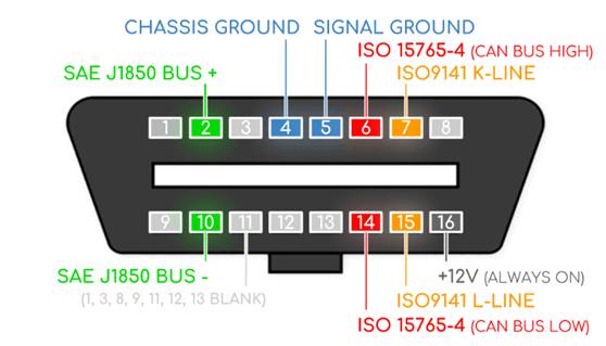
The OBD2 system can be accessed via an OBD2 16-pin connector found within 0.61m of the steering wheel.
OBD System Gives Vehicle Technician Access to Health Information for
Vehicle Sub System
Standards specified by
OBD
Type of diagnostic connectors and pin-out
Protocols supported
Messaging format
How OBD II Works
Modern Electronics With Self Diagnosis supports The Technician by Registering actual Values ,comparing Them with Nominal Values & Diagnosing Faults that are Stored for Repair Purpose
There are many sensors throughout your car: oxygen sensors, engine knock sensors, manifold pressure sensors and so on and so on. Each one of these sensors sends a signal to your car’s computer the Engine Control Unit (ECU). The ECU uses that information to adjust different elements of your engine operation, the fuel injection or the spark timing for example.
During the Operating Time of The vehicle ECU’s are Constantly checking the sensors they are connected to.By Comparing the Measured Values and Stored data an ECU is able to Determine whether Measured Values exceed or still within Tolerance Required
If the information that the ECU gets from one of its sensors is too far out of whack, it saves a code called a Diagnostic Trouble Code (DTC). It also sends a signal to you check engine light. If the light comes on and stays on, then you have a minor problem
This Fault Memory can be Read Later in workshop and Provide Valuable information for The Technician.
OBD communication protocols
OBD regulations are defined by a series of SAE/ISO standards, that describe in detail how certain OBD functions need to be implemented on the ECU side, and how the communication between the ECU and the diagnostic tool is going to be performed.
OBD-2 (US) regulations are described in SAE standards, EOBD (EU) regulations are described in ISO standards.
The OBD communication protocol can be regarded as an OSI (Open Systems Interconnection) model, with several layers, each defined in a standard:
OBD means also data exchange between vehicle and external equipment (scantool). This can be done using on of the following protocols:
Protocol
Description
SAE J1850 PWM
Pulse Width Modulation used mainly by Ford Motor Company data transfer speed 41.6 kBaud/s uses two wires for data transmission
SAE J1850 VPW
Variable Pulse Width used mainly by General Motors data transfer speed between 10.4 and 41.6 kBaud/s uses two wires for data transmission
ISO 9141-2
Used mainly by Chrysler, European and Asian vehicle manufacturers data transfer speed 10.4 kBaud/s. uses only one wire for data transmission (K-line), the second line (L-line) is optional
ISO 14230 (KWP2000)
KeyWord Protocol similar with ISO 9141-2 data transfer speed between 1.2 and 10.4 kBaud/s. uses only one wire for data transmission (K-line), the second line (L-line) is optional
ISO 15765 (CAN)
Controller Area Network starting with 2008 all new vehicles sold in USA must use CAN as OBD communication protocol starting with Euro 4 most of the vehicles sold in EU use CAN as OBD communication protocol data transfer speed between 250 and 500 k Baud/s uses two wires for data transmission (CAN-high and CAN-low)
On-Board Diagnostics (OBD) – introduction to the Modes of Operation (Diagnostic Services)
OBD modes of operation (also called diagnostic services) define how the data is requested from the vehicle and how the vehicle responds to the request. You can look at the OBD modes of operation as a definition of the “language” to be used by both parties (scan tool and vehicle) when requesting and sending data.
The diagnostic Service can be defined as an information exchange initiated by a client (external test equipment) in order to require diagnostic information from a server (ECU) or/and to modify its behaviour for diagnostic purpose.
In the OBD CAN protocol there are 9/10 modes of operation (diagnostic services), each defined by an identifier (also called header). First 9 modes of operation are common between ISO and SAE standards, the 10th is specific to the SAE standard.
The communication between diagnostic device (scantool) and vehicle is client-server type, based on request and response.
The Client is defined as the function that is part of the diagnostic device (scantool, tester), that makes use of the diagnostic services .
The Server is defined as a function that is part of an electronic control unit on-board of the vehicle and that provides data to the diagnostic services.
The diagnostic Service can be defined as an information exchange initiated by a client (external test equipment) in order to require diagnostic information from a server (ECU) or/and to modify its behavior for diagnostic purpose.
The table below describes the purpose of each mode of operation (diagnostic service) and which standard contains it
Diagnostic service Mode of operation
Description
Standard
$01
Request Current Powertrain Diagnostic Data
SAE, ISO
$02
Request Powertrain Freeze Frame Data
SAE, ISO
$03
Request Emission-Related Diagnostic Trouble Codes
SAE, ISO
$04
Clear/Reset Emission-Related Diagnostic Information
SAE, ISO
$05
Request Oxygen Sensor Monitoring Test Results
SAE, ISO
$06
Request On-Board Monitoring Test Results for Specific Monitored Systems
SAE, ISO
$07
Request Emission-Related Diagnostic Trouble Codes Detected During Current or Last Completed Driving Cycle
SAE, ISO
$08
Request Control of On-Board System, Test or Component
SAE, ISO
$09
Request Vehicle Information
SAE, ISO
$0A
Request Emission-Related Diagnostic Trouble Codes with Permanent Status
SAE
The dollar sign “$” in front of the numerical value highlights that this is an identifier. It’s important to know that the numerical values of the identifiers are in hexadecimal format
OBD2 PIDS & MESSAGES EXPLAINED:
In simplified terms, an OBD2 message is comprised of an identifier and data.
An example of a request/response CAN message for the PID ‘Vehicle Speed’
with a value of 50 km/h can look like this:
Request: 7DF 02 01 0D 55 55 55 55 55
Response: 7E8 03 41 0D 32 aa aa aa aa
(Here the 32 is the hexadecimal value of 50).
IDENTIFIER: For OBD2 messages, the identifier is standard 11-bit and used to distinguish between “request messages” (ID 7DF) and “response messages” (ID 7E8 to 7EF). Note that 7E8 will typically be where the main engine or ECU responds at.
LENGTH: This simply reflects the length in number of bytes of the remaining data (03 to 06). For the Vehicle Speed example, it is 02 for the request (since only 01 and 0D follow), while for the response it is 03 as both 41, 0D and 32 follow.
MODE: For requests, this will be between 01-0A. For responses the 0 is replaced by 4 (i.e. 41, 42, … , 4A). There are 10 modes as described in the SAE J1979 OBD2 standard. Mode 1 shows Current Data and is e.g. used for looking at real-time vehicle speed, RPM etc. Other modes are used to e.g. show or clear stored diagnostic trouble codes and show freeze frame data.
PID: For each mode, a list of standard OBD2 PIDs exist – e.g. in Mode 01 PID 0D is Vehicle Speed. For the full list, check out the aforementioned Wikipedia OBD2 PID overview. Each PID has a description and some have a specified minimum/maximum and conversion formula.
The formula for speed is e.g. simply A, meaning that the Ah data byte (which is in HEX) is converted to decimal to get the km/h converted value (i.e. 32 becomes 50 km/h above). For e.g. RPM (PID 0C), the formula is (256*A + B) / 4.
Ah, Bh, Ch, Dh: These are the data bytes in HEX, which need to be converted to decimal form before they are used in the PID formula calculations. Note that the last data byte (after Dh) is not used.
HOWTO LOG OBD2 DATA?
OBD2 data logging works as follows:
You connect a OBD2 scanner or OBD2 data logger to the OBD2 16 pin connector
Via the tool, you enter “request messages” (queries) transmitted via the CAN-bus
The relevant ECUs react and send “response messages” via the CAN-bus
When you attach an
OBD-II scan tool, it sends specially formatted diagnostic command messages over
the CAN bus. Nodes on the network that can output diagnostic information are
listening for these messages, and send out the requested status information
over CAN when asked. For example the technician enters Mode 1 (query the real
time state of the car, meaning your car needs to be started) PID 0D (query for
vehicle speed) into the scan tool, and the scan tool sends the corresponding
message over the CAN bus, and the engine control unit that knows the vehicle
speed returns the vehicle speed (the response format is defined by OBD-II PIDs
at http://en.wikipedia.org/wiki/OBD-II_PIDs), and the scan tool displays the
vehicle speed on the tool’s screen.
THE OBD-2 CONNECTOR
The OBD2 standard (SAE J1962) specifies two female OBD2 16-pin connector types (A & B). Below is an example of a Type A OBD2 pin connector (also sometimes referred to as the Data Link Connector
Exploring the Scope of Off-board Diagnostics in the Vehicle
Off-board vehicle diagnostics takes care of the diagnostics of every other vehicle ECU function other than emission. There are several protocol standards defined for off-board diagnostics, however,
Unified Diagnostics Services (UDS) is the most popular diagnostic protocol. The diagnostics manager of the UDS protocol stores every issue as fault codes called Diagnostics Trouble Code (DTC). When a vehicle is running, the off-board diagnostics is also active. However, the contrast with on-board diagnostics lies in the reporting part.
In case of OBD, the fault is communicated to the information cluster by triggering the Malfunction indicator light. Whereas, in the off board diagnostics, no such instant reporting is carried out. The issue is stored in the EEPROM part of the vehicle ECU for retrieval at the service garage using a vehicle diagnostic testing tool.
However, the scope of off-board diagnostics (UDS) is not limited to just storing the diagnostic trouble codes (DTCs). It is capable of offering services such as vehicle ECU reprogramming, remoteroutine activation, writing data on the automotive Electronic Control Unit and even more.
This is one of the major aspects that differentiates on-board and off board vehicle diagnostics. When the UDS stack is integrated to the vehicle ECU, the UDS services are configured to it. These configurations are mostly OEM specific. It means that a tester tool authorized by the same automotive OEM can only read or write data from the vehicle ECU. Unlike the OBD 2, any after-market tester tool will not work.
Services
As UDS has been accepted by many automotive OEMs as the de facto Off-board diagnostics, its services are very important. We have compiled them here:
UDS ServicesDescription
0x10 Diagnostic Session Enable various diagnostics sessions Control within ECU
0x11 ECU Reset Resetting the ECU to be back in the default session
0x27 Security Access Limit access to data and services to prevent unauthorized access
0x3E Tester Present Alert the ECU(s) that client is still connected so that diagnostic sessions remain active.
0x22 Read Data By Identifier Request data from ECU(s)
0x2E Write Data By Identifier Write data onto ECU(s)
0x14 Clear Diagnostic Information Clear diagnostic trouble codes (DTC) stored in the ECU
0x19 Read DTC Information Read DTC from the ECU
0x2F Input Output Control By Identifier Control the input/output signals through the diagnostic interface
0x31 Routine Control control all the routine services (erasing memory, testing routines etc.)
0x34 Request Download Request ECU to initiate download session based on request from the tester
On-board Vs Off-board Vehicle Diagnostics: A QuickComparison
scope and services of both on-board and off-board vehicle diagnostics should be clear by now. Emission being a very crucial aspect of a vehicle, on-board diagnostics is completely dedicated to it. The strict CARB and EURO emission guidelines call for real-time monitoring of emission related parameters. The Malfunction Indicator light is also associated with the on-board diagnostics, implying the urgency an emission related issue requires. The off-board vehicle diagnostics, on the other hand, may not require enough urgency to light up an MIL. However, it has many other roles to play. Its comprehensive set of services help the garage personnel perform tests, run routines, update the ECU, write data and much more.
The crux of the story is that both on-board and off-board systems perform diagnostics and have their scope clearly demarcated by their services. While one takes care of the emission the other handles everything other than that
The difference between UDS and OBD protocols
UDS (Unified Diagnostic Services) is a diagnostic communication protocol in the electronic control unit (ECU) environment within the automotive electronics. It is similar to ISO 14230-3 (KWP2000) and ISO 15765-3 (Diagnostic Communication over Controller Area Network (DoCAN)). The protocol is “unified” in the sense that it is used internationally across different companies and manufacturers. UDS differs from the CAN protocol in a crucial way. The CAN protocol specifies the first and second layer of the OSI Model – that is the Physical Layer (ISO 11898-2) and the Data Link Layer (ISO 11898-1). UDS, however, also specifies the fifth (Session Layer) and seventh (Application Layer) layers of the OSI Model.
OBD (On-board diagnostics) is an automotive term referring to a vehicle’s self-diagnostic and reporting capability. OBD systems give the vehicle owner or repair technician access to the status of the various vehicle subsystems. It is used to implement vehicle diagnostics communication for diagnosis and repair of vehicle sub-systems through communication with Electronic Control Units (ECU). ECUs monitor and control the sub-systems of a vehicle. Common ECUs include Engine Control Module (ECM), Transmission Control Module (TCM), Electronic Brake Control Module (EBCM), etc. Thus OBD helps to detect and control engine failures, performance issues and fight vehicle emission. Generally, UDS and OBD are both diagnostic protocol, but they are actually not comparable. While UDS protocol is used to diagnose a fault in an off-board condition, i.e. when the car is at the service center, OBD is essentially an onboard diagnostic service.
Link between OBD2 and CAN bus
On board diagnostics, OBD2, is a ‘higher layer protocol‘ (like a language). CAN is a method for communication (like a phone).
In particular, the OBD2 standard specifies the OBD2 connector, incl. a set of five protocols that it can run on (see below). Further, since 2008, CAN bus (ISO 15765) has been the mandatory protocol for OBD2 in all cars sold in the US.
What is the ISO 15765 standard?
ISO 15765 refers to a set of restrictions applied to the CAN standard (which is itself defined in ISO 11898). One might say that ISO 15765 is like “CAN for cars”.
In particular, ISO 15765-4 describes the physical, data link layer and network layers, seeking to standardize the CAN bus interface for external test equipment. ISO 15765-2 in turn describes the transport layer (ISO TP) for sending CAN frames with payloads that exceed 8 bytes. This sub standard is also sometimes referred to as Diagnostic Communication over CAN (or DoCAN). See also the 7 layer OSI model illustration.
So This was Brief Introduction to Diagnostics in Next Blog we will learn about CAN Protocol.
What is Unified Diagnostic Service (UDS) Protocol?
With rapid implementation of electronic embedded systems in vehicles, the need to track and control the vehicle’s different parameters was imperative. Thus, diagnostic systems were developed so that the clients (designers, testers, and mechanics) could detect the faults in the vehicle by connecting their diagnostic tester tool to the electronic control units (ECUs) in the vehicle.
Unified Diagnostic Service (UDS) is an automotive protocol that lets the diagnostic systems communicate with the ECUs to diagnose faults and reprogram the ECUs accordingly (if required).
UDS is called “Unified” because it combines and consolidates standards such as KWP 2000 (ISO 14230) or Diagnostics on CAN (ISO 15765) and is independent of vehicle manufacturers.
ISO-14229 Standards Available:
ISO-14229 consists of the following parts, under the general title Road vehicles — Unified diagnostic services (UDS):
ISO 14229-1: Specification and requirements.
ISO 14229-2: Session layer services.
ISO 14229-3: Unified diagnostic services on CAN implementation (UDSonCAN).
ISO 14229-4: Unified diagnostic services on FlexRay implementation (UDSonFR).
ISO 14229-5: Unified diagnostic services on Internet Protocol implementation (UDSonIP).
ISO 14229-6: Unified diagnostic services on K-Line implementation (UDSonK-Line).
Need for UDS Protocol for Vehicle Diagnostics
As OEM’s integrate/assemble automotive ECU and components from different suppliers, a need for a standard diagnostic protocol was felt.
This is because, prior to a Unified Protocol OEMs’ and suppliers had to deal with compatibility issues between different diagnostic protocols like KWP 2000, ISO 15765, and diagnostics over K-Line.
Unified Diagnostic Service (UDS) is the preferred choice of protocols for all the off-board vehicle diagnosis. Off-board diagnostics refers to the diagnostics of the vehicle parameters when the car is at servicing in the garage (when the car is stationary).
ECU flashing and reprogramming can also be performed efficiently with the help of UDS protocol stack.
Also, UDS protocol is quite flexible and is capable of performing more detailed diagnostics as compared to other protocols like OBD and J1939.
Implementation of UDS on CAN in OSI model
The diagnostic tool contacts all control units installed in a vehicle, which have UDS services enabled. In contrary to the CAN protocol, which only uses the first and second layers of the OSI Model, UDS services utilize the fifth and seventh layers of the OSI model.
The messages defined in UDS can be sent to the controllers which must provide the predetermined UDS services. This makes it possible to inteograte the fault memory of the individual control units or to update them with a new firmware.
ISO 14229-1 has been established in order to define common requirements for diagnostic systems, whatever the serial data link is.
ISO 15765-2, or ISO-TP is an international standard for sending data packets over a CANBus. – The protocol allows for the transport of messages that exceed the eight byte maximum payload of CAN frames. – ISO-TP segments longer messages into multiple frames, adding metadata that allows the interpretation of individual frames and reassembly into a complete message packet by the recipient. – It can carry up to 4095 bytes of payload per message packet.
What is the difference between UDS protocol and OBD protocol?
Although UDS and OBD2 are both diagnostic protocol, they are actually not comparable. While UDS protocol is used to diagnose fault in an off-board condition, i.e. when the car is at the service center, OBD is essentially an on-board diagnostic service.
However, I will try to draw some comparison to clear the air.
1. OBD2 is essentially used for emission related diagnosis of the vehicle which implies that it interacts only with those ECUs that control emission.
UDS Protocol on the other hand is ideal for both emission and non-emission related diagnosis.
2. The next difference is in terms of layers. OBD 2 has 4 layers viz. application layer, transport layer, data link layer, and the physical layer.
UDS protocol is defined in the ISO 14229 standard. It is the application layer of the OSI reference model and is independent of the bus-system. The protocols for specific bus-systems like CAN and K-Line etc. are defined in separate standards viz. ISO 15765-3 (CAN). This way, the OEMs are not bound to use any specific communication system in the vehicle.
The messages and data in OBD2 are defined in the protocol and cannot be modified by the OEMs. However, UDS protocol gives the OEMs the liberty to specify how they define the data as well as the parameters.
Physical and functional addressing:
There is a possibility for the diagnostic tester (client) to send physical or functional UDS-requests. A functional request is a broadcast-type message which will be sent to all ECU:s which are on the CAN-network. Physical the UDS-requests are only sent to a single ECU on the network. Suppose already you know in which module or ECU the faults are happening, then the diagnostic engineer in the service center can directly connect to that ECU to send the diagnostic request (Physical addressing) and read the diagnostic data and fix the issue. If the engineer don’t know where is the fault happening obviously he will be sending the request (Functional addressing) globally to all the ECU available in the vehicle, read all the active DTC and fix it.
UDS Diagnostic Frame Format:
Since the UDS protocol is working on the CAN protocol so that the maximum 8-bytes of the data can be requested and get to the response in a message. Like CAN protocol, in UDS protocol, there are 2-types of the frames are available.
Again the Response frame is divided into two types as:
Positive Response.
Negative Response
UDS Protocol Request Frame Format:
Whenever the client wants to request anything from the data then the tester will send this request the frame to get the response from the server on the CAN data field. This frame had consisted of 3 fields as:
Service ID. Sub-Function ID (optional: not exist for some diag. services).
Whenever a diagnostic engineer or tester will request any service to a vehicle, there is a possibility of two types of response from the vehicle or from a particular ECU as per physical or functional request type.
Positive Response Frame Format:
Whenever the tester will request to the server if it is correct and the server has been executed the request successfully, then it will send to the response message with respect to this request by the adding 0x40 to the respective service ID for the reference. Positive response 1st byte should be Request Service ID + 0x40.
onse frame else it will be a -Ve response message with Negative Response Code (NRC)
UDS message structure
UDS is a request based protocol. In the illustration we’ve outlined an example of an UDS request frame (using CAN bus as basis):
#1 Protocol Control Information (PCI)
The PCI field is not per se related to the UDS request itself, but is required for diagnostic UDS requests made on CAN bus. In short, the PCI field can be 1-3 bytes long and contains information related to the transmission of messages that do not fit within a single CAN frame. We will detail this more in the section on the CAN bus transport protocol (ISO-TP).
#2 UDS Service ID (SID)
The use cases outlined above relate to different UDS services. When you wish to utilize a specific UDS service, the UDS request message should contain the UDS Service Identifier (SID) in the data payload. Note that the identifiers are split between request SIDs (e.g. 0x22) and response SIDs (e.g. 0x62). As in OBD2, the response SIDs generally add 0x40 to the request SIDs.
#3 UDS Sub Function Byte
The sub function byte is used in some UDS request frames as outlined below. Note, however, that in some UDS services, like 0x22, the sub function byte is not used.
Generally, when a request is sent to an ECU, the ECU may respond positively or negatively. In case the response is positive, the tester may want to suppress the response (as it may be irrelevant). This is done by setting the 1st bit to 1 in the sub function byte. Negative responses cannot be suppressed.
The remaining 7 bits can be used to define up to 128 sub function values. For example, when reading DTC information via SID 0x19 (Read Diagnostic Information), the sub function can be used to control the report type – see also below table.
Negative Response Frame Format:
If the client did not request in a proper frame format or the server is not able to execute the request due to the internal problem, then it will send the negative response to the client. Negative response 1st byte should be 0x7F. Negative response 2nd byte should be Service ID. Negative response 3rd byte should be Response Code.
In the above table i have give a demo request and response message format. Like this if any diagnostic data needed the tester can request from his computer to the vehicle or you can say a particular ECU to get the data as response message. If the request will received by the ECU or server successfully and executed also with all the preconditions then the ECU or server will send the message with +Ve resp
When an ECU responds positively to an UDS request, the response frame is structured with similar elements as the request frame. For example, a ‘positive’ response to a service 0x22 request will contain the response SID 0x62 (0x22 + 0x40) and the 2-byte DID, followed by the actual data payload for the requested DID. Generally, the structure of a positive UDS response message depends on the service.
However, in some cases an ECU may provide a negative response to an UDS request – for example if the service is not supported. A negative response is structured as in below CAN frame example:
Below we briefly detail the negative response frame with focus on the NRC:
The 1st byte is the PCI field
The 2nd byte is the Negative Response Code SID, 0x7F
The 3rd byte is the SID of the rejected request
The 4th byte is the Negative Response Code (NRC)
In the negative UDS response, the NRC provides information regarding the cause of the rejection as per the table below.
Functions of Diagnostic Services
Besides specifying services’ primitives and protocols that describe the client-server interaction, UDS also defines within its framework a number of functional units that comprise several services each, identified with a hexadecimal code. These units are intended for the different individual purposes that support the overall diagnostic function/task. The UDS protocol having different services for the different types of work tasks to do on the server. These are having 6- types as: 1. Diagnostic and communication management. 2. Data Transmission. 3. Stored Data Transmission. 4. Input/Output Control. 5. Remote activation of routine. 6. Upload/Download.
Diagnostic and communication management:
There are 10 services are available in this module to control the diagnostic and the communication-related in the ECU.
1. Diagnostic Session Control (0x10)
2. ECU Reset (0x11)
3. Security Access (0x27)
4. Communication Control (0x28)
5. Tester Present (0x3E)
6. Access Timing Parameter (0x83)
7. Secure Data Transmission (0x84)
8. Control DTC setting (0x85)
9. Response To Event (0x86)
10. Link Control (0x87)
Function group
Request SID
Response SID
Service
Description
Diagnostic and Communications Management
$10
$50
Diagnostic Session Control
UDS uses different operating sessions, which can be changed using the “Diagnostic Session Control”. Depending on which session is active, different services are available. On start, the control unit is by default in the “Default Session”. Other sessions are defined, but are not required to be implemented depending on the type of device:”Programming Session” used to upload software.”Extended Diagnostic Session” used to unlock additional diagnostic functions, such as the adjustment of sensors.”Safety system diagnostic session” used to test all safety-critical diagnostic functions, such as airbag tests.In addition, there are reserved session identifiers that can be defined for vehicle manufacturers and vehicle suppliers specific use.
$11
$51
ECU Reset
The service “ECU reset” is used to restart the control unit (ECU). Depending on the control unit hardware and implementation, different forms of reset can be used:”Hard Reset” simulates a shutdown of the power supply.”key off on Reset” simulates the drain and turn on the ignition with the key.”Soft Reset” allows initialization of certain program units and their storage structures.Again, there are reserved values that can be defined for vehicle manufacturers and vehicle suppliers specific use.
$27
$67
Security Access
Security check is available to enable the most security-critical services. For this purpose a “Seed” is generated and sent to the client by the control unit. From this “Seed” the client has to compute a “Key” and send it back to the control unit to unlock the security-critical services.
$28
$68
Communication Control
With this service, both the sending and receiving of messages can be turned off in the control unit.
$3E
$7E
Tester Present
If no communication is exchanged with the client for a long time, the control unit automatically exits the current session and returns to the “Default Session” back, and might go to sleep mode. Therefore, there is an extra service which purpose is to signal to the device that the client is still present.
$83
$C3
Access Timing Parameters
In the communication between the controllers and the client certain times must be observed. If these are exceeded, without a message being sent, it must be assumed that the connection was interrupted. These times can be called up and changed.
$84
$C4
Secured Data Transmission
$85
$C5
Control DTC Settings
Enable or disable the detection of any or all errors. This is important when diagnostic work is performed in the car, which can cause an anomalous behavior of individual devices.
$86
$C6
Response On Event
$87
$C7
Link Control
The Service Link Control is used to set the baud rate of the diagnostic access. It is usually implemented only at the central gateway.
Data Transmission
$22
$62
Read Data By Identifier
With this service it is possible to retrieve one or more values of a control unit. This can be information of all kinds and of different lengths such as Partnumber or the software version. Dynamic values such as the current state of the sensor can be queried. Each value is associated to a Data Identifier (DID) between 0 and 65535. Normal CAN signals are meant for information that some ECU uses in its functionality. DID data is sent on request only, and is for information that no ECU uses, but a service tool or a software tester can benefit from.
$23
$63
Read Memory By Address
Read data from the physical memory at the provided address. This function can be used by a testing tool, in order to read the internal behaviour of the software.
$24
$64
Read Scaling Data By Identifier
$2A
$6A
Read Data By Identifier Periodic
With this service values are sent periodically by a control unit. The values to be sent must be defined to only using the “Dynamically Define Data Identifier”.
$2C
$6C
Dynamically Define Data Identifier
This service offers the possibility of a fix for a device specified Data Identifier (DID) pool to configure another Data Identifier. This is usually a combination of parts of different DIDs or simply a concatenation of complete DIDs.The requested data may be configured or grouped in the following manner:Source DID, position, length (in bytes), Sub-Function Byte: defineByIdentifierMemory address length (in bytes), Sub-Function Byte: defineByMemoryAddressCombinations of the two above methods through multiple requests.
$2E
$6E
Write Data By Identifier
With the same Data Identifier (DID), values can also be changed. In addition to the identifier, the new value is sent along.
$3D
$7D
Write Memory By Address
Stored Data Transmission
$14
$54
Clear Diagnostic Information
Delete all stored DTC
$19
$59
Read DTC Information
control unit fault is stored with its own code in the error memory and can be read at any time. In addition to the error, additional information will be stored, which can also be read.
Input / Output Control
$2F
$6F
Input Output Control By Identifier
This service allows an external system intervention on internal / external signals via the diagnostic interface.By specifying a so-called option bytes additional conditions for a request can be specified, the following values are specified:ReturnControlToECU: The device must get back controls of the mentioned signals.ResetToDefault: The tester prompts to reset signals to the system wide default value.Freeze Current State: The device shall freeze the current signal value.ShortTermAdjustment: The device shall use the provided value for the signal
Remote Activation of Routine
$31
$71
Routine Control
The Control service routine services of all kinds can be performed. There are three different message types:With the start-message, a service can be initiated. It can be defined to confirm the beginning of the execution or to notify when the service is completed.With the Stop message, a running service can be interrupted at any time.The third option is a message to query the results of the service.The start and stop message parameters can be specified. This makes it possible to implement every possible project-specific service.
Upload / Download
$34
$74
Request Download
Downloading new software or other data into the control unit is introduced using the “Request Download”. Here, the location and size of the data is specified. In turn, the controller specifies how large the data packets can be.
$35
$75
Request Upload
The service “request upload” is almost identical to the service “Request Download”. With this service, the software from the control unit is transferred to the tester. The location and size must be specified. Again, the size of the data blocks are specified by the tester.
$36
$76
Transfer Data
For the actual transmission of data, the service “Transfer Data” is used. This service is used for both uploading and downloading data. The transfer direction is notified in advance by the service “Request Download” or “Upload Request”. This service should try to send packets at maximum length, as specified in previous services. If the data set is larger than the maximum, the “Transfer Data” service must be used several times in succession until all data has arrived.
$37
$77
Request Transfer Exit
A data transmission can be ‘completed’ when using the “Transfer Exit” service. This service is used for comparison between the control unit and the tester. When it is running, a control unit can answer negatively on this request to stop a data transfer request. This will be used when the amount of data (set in “Request Download” or “Upload Request”) has not been transferred.
$38
$78
Request File Transfer
This service is used to initiate a file download from the client to the server or upload from the server to the client. Additionally information about the file system are available by this service.
$7F
Negative Response
This response is given when a service request could not be performed, for example having a not supported Data Identifier. A Negative Response Code will be included.
UDS vs CAN bus: Standards & OSI model
To better understand UDS, we will look at how it relates to CAN bus and the OSI model.
Overview of UDS standards & concepts
The ISO 14229-1 standard describes the application layer requirements for UDS (independent of what lower layer protocol is used). In particular, it outlines the following:
Client-server communication flows (requests, responses, …)
UDS services (as per the overview described previously)
Positive responses and negative response codes (NRCs)
Various definitions (e.g. DTCs, parameter data identifiers aka DIDs, …)
The purpose of 14229-3 is to enable the implementation of Unified Diagnostic Services (UDS) on Controller Area Networks (CAN) – also known as UDSonCAN. This standard describes the application layer requirements for UDSonCAN.
This standard does not describe any implementation requirements for the in-vehicle CAN bus architecture. Instead, it focuses on some additional requirements/restrictions for UDS that are specific to UDSonCAN
Specifically, 14229-3 outlines which UDS services have CAN specific requirements. The affected UDS services are ResponseOnEvent and ReadDataByPeriodicIdentifier, for which the CAN specific requirements are detailed in 14229-3. All other UDS services are implemented as per ISO 14229-1 and ISO 14229-2.
ISO 14229-3 also describes a set of mappings between ISO 14229-2 and ISO 15765-2 (ISO-TP) and describes requirements related to 11-bit and 29-bit CAN IDs when these are used for UDS and legislated OBD as per ISO 15765-4.
This describes the session layer in the UDS OSI model. Specifically, it outlines service request/confirmation/indication primitives. These provide an interface for the implementation of UDS (ISO 14229-1) with any of the communication protocols (e.g. CAN).
For UDS on CAN, ISO 15765-2 describes how to communicate diagnostic requests and responses. In particular, the standard describes how to structure CAN frames to enable communication of multi-frame payloads. As this is a vital part of understanding UDS on CAN, we go into more depth in the next section.
When UDS is based on CAN bus, the physical and data link layers are described in ISO 11898-1 and ISO 11898-2. When UDS is based on CAN, it can be compared to a higher layer protocol like J1939, OBD2, CANopen, NMEA 2000 etc. However, in contrast to these protocols, UDS could alternatively be based on other communication protocols like FlexRay, Ethernet, LIN etc.
CAN ISO-TP – Transport Protocol (ISO 15765-2)
When implementing diagnostics on CAN, one challenge is the size of the CAN frame payload: For Classical CAN frames, this is limited to 8 bytes and for CAN FD the payload is limited to 64 bytes. Vehicle diagnostics often involves communication of far larger payloads.
ISO 15765-2 was established to solve the challenge of large payloads for CAN based vehicle diagnostics.
The standard specifies a transport protocol and network layer services for use in CAN based vehicle networks.
The ISO-TP standard outlines how to communicate CAN data payloads up to 4095 bytes through segmentation, flow control and reassembly. ISO-TP defines specific CAN frames for enabling this communication as shown below:
ISO-TP: Single-frame communication
In vehicle diagnostics, communication is initiated by a tester tool sending a request. This request frame is a Single Frame (SF).
In the simplest case, a tester tool sends a Single Frame to request data from an ECU. If the response can be contained in a 7-byte payload, the ECU provides a Single Frame response.
ISO-TP: Multi-frame communication
When the payload exceeds 7 bytes, it needs to be split across multiple CAN frames.
As before, a tester starts by sending a Single Frame (SF) request to an ECU (sender). However, in this case the response exceeds 7 bytes.
Because of this, the ECU sends a First Frame (FF) that contains information on the total packet length (8 to 4095 bytes) as well as the initial chunk of data.
When the tester receives the FF, it will send a Flow Control (FC) frame, which tells the ECU how the rest of the data transfer should be transmitted.
Following this, the ECU will send Consecutive Frames (CF) that contain the remaining data payload.
Security Access Service Identifier (0x27): UDS Protocol
To prevent the ECU is modified by unauthorized persons most UDS services are locked. To get access to services that are used to modify the ECU the user first has to grant access through the Security Access Service Identifier (0x27). Only after the security access service has been passed, services like Request Download and Transfer Data can be used. The security concept used is called “Seed and Key”. Security Access Service flow:
The client sends a request for a “seed” to the server that it wants to unlock.
The server replies by sending the “seed” back to the client.
The client then generates a “key” based on the “seed” and sends the key to the server.
If the client generated the “key” with the correct algorithm the server will respond that the “key” was valid and that it will unlock itself.
Security Access Seed Request Frame
The above table defines what data format should be maintained to use the Security Access service in UDS Protocol for requesting a seed. Let me explain to you one example of how to request a seed:
Security Access Seed Response Frame
The response message has a response SID and if it is a positive response the parameter is an echo of the request message parameter. If it is a negative response the parameter is one of eight negative response codes.
In past electronic devices in vehicles are connected via point to point wiring system.
More Electronic in vehicle which resulted in bulky wire harnesses that were expensive and heavy too and if new nodes need to be introduced, it will be very difficult and complex.
In electronic systems signals are sent from one chip to another using wires (let’s forget about wireless things for a second). The simplest way of doing so is to use one wire per bit of information you like to transmit. One bit of information is simply an answer to a yes/no question like “Are the headlights on?” If the headlights are on, there is a voltage on that wire, say 5 volts. If they are off there are 0 volts on the wire.
Now that’s fine for one bit of information. But more data requires more wires. Unfortunately: More wires means more complexity. A modern car is just a computer with wires on it, so there are a lot of wires (several km or miles) in it. More wires result in more weight and more costs and car manufacturers don’t like that. So we need a way to reduce the amount of wires.
The usual way of doing so is to use a bus system.
Think of a bus as a way to transmit more information using fewer wires.
So Vehicle Bus is an internal communication network that interconnects components inside a vehicle
What are the difference between an OBD-II protocol and a CAN setup?
OBD-II is a higher-level protocol used for diagnostic purposes. OBD-II can use one of (many) different bus systems to transfer diagnostic data from and to your car. Think of OBD-II as a language (English) that you speak and of CAN as the communication device (telephone) you use to talk to someone (about your car and its state of health.
What is CAN?
CAN (Controller Area Network) is a serial bus system, which was originally developed for automotive applications in the early 1980’s.
The CAN bus was developed by BOSCH (1) as a multi-master, message broadcast system that specifies a maximum signaling rate of 1 megabit per second (bps).
CAN is a two-wire, half duplex, high-speed network system, that is far superior to conventional serial technologies such as RS232 in regards to functionality and reliability and yet CAN implementations are more cost effective
The CAN bus is a broadcast type of bus. This means that all nodes can “hear” all transmissions. There is no way to send a message to just a specific node; all nodes will invariably pick up all traffic.
Unlike a traditional network such as USB or Ethernet, CAN does not send large blocks of data point-to-point from node A to node B under the supervision of a central bus master.
CAN Bus Explained with an Analogy
Imagine that your car is like a human body:
The Controller Area Network (CAN bus) is the nervous system, enabling communication between all parts of the body.
Similarly, ‘nodes’ are like muscles connected via the CAN bus, which acts as a central networking system. In turn, electronic control units (ECU) are like arms and legs.
Each of the devices on the network has a CAN controller chip and is therefore intelligent. All transmitted messages are seen by all devices on the network. Each device can decide if the message is relevant or if it can be filtered.
Specifications:
· Provides better ease of use than any other serial bus system
· Operates at data rates of up to 1 Megabit per second
· Has excellent error detection and fault confinement capabilities
• Up to 1 Mbit/s at cable length 40 m
• 0 – 8 bytes of data/frame
• Event triggered, messages are sent when there is something to send
– Practical limit is approximately 100 nodes due to transceiver
– Most buses use 3–10 nodes
CAN Standard
CAN is an International Standardization Organization (ISO) defined serial communications bus originally developed for the automotive industry to replace the complex wiring harness with a two-wire bus.
The CAN communications protocol, ISO-11898: , describes how information is passed between devices on a network and conforms to the Open Systems Interconnection (OSI) model that is defined in terms of layers
The data link layer protocol defined by ISO 11898-1 and the physical layer defined by ISO 11898-2.
The ISO 11898 architecture defines the lowest two layers of the seven layer OSI/ISO model as the data-link layer and physical layer
CAN Working Principle
CAN is multi master message model Any node can transmit or receive any message
Data transmitted From any Node on CAN bus Nodes does not contain Addresses of either the transmitting Node or any intended receiving Node instead it contains Message Which will be labelled By an Identifier
All Other Nodes Receive the message & Perform an acceptance test on the identifier to determine if the message & thus its content is relevant to that Particular Node
If Message is relevant it will be Processed Otherwise It is Ignored
What is meant when referring to a physical layer, or an application layer?
The International Organization for Standardization (ISO) developed the Open System Interconnect (OSI) model in 1984 as a model of computer communication architecture. There are seven layers to the OSI model: Physical, Data Link, Network, Transport, Session, Presentation, and Application. The intent is that protocols be developed to perform the functions of each layer as needed.
The OSI layer model
Layer1 –
The physical layer transmits bit from one device to another and regulates the transmission of bit streams. It defines the specific voltage and the type of cable to be used for transmission protocols. It provides the hardware means of sending and receiving data on a carrier defining cables, cards and physical aspects.
Layer 2 – Data link layer Converts data frames from the bits on the wire to packages that the network layer can handle It packages raw data into frames transferred from physical layer. This layer is responsible for transferring frames from one device to another without errors. After sending the frame it waits for the acknowledgement from receiving device. Data link layer has two sub layers:
MAC (Medium Access Control) layer: It performs frame coding, error detection, signaling, serialization and de-serialization.
LLC (Logical Link Control) layer: The LLC sub layer provides multiplexing mechanisms that make it possible for several network protocols (IP, Decnet and Appletalk) to coexist within a multipoint network and to be transported over the same network medium. It performs the function of multiplexing protocols transmitted by MAC layer while transmitting and decoding when receiving and providing node-to-node flow and error control.
Layer 3 – Network layer Handles data paths. Converts logical addresses to physical addresses It provides end to end logical addressing system so that a packet of data can be routed across several layers and establishes, connects and terminates network connections.
Layer 4 –The transport layer ensures that messages are delivered error-free, in sequence, and without loss or duplication. It relieves the higher layer from any concern with the transfer of data between them and their peers.
Layer5– It allows to establishing, communicating and terminating sessions between processes running on two different devices performing security, name recognition and logging.
Layer 6 – Presentation layer Converts between the data format of the application and the data format of the network The most important function of this layer is defining data formats such as ASCII text, EBCDIC text BINARY, BCD and JPEG. It acts as a translator for data into a format used by the application layer at the receiving end of the station.
Layer 7 –Application layer It serves as a window for users and application processes to access network services. The common functions of the layers are resource sharing, remote file access, network management, electronic messages and so on.
CAN protocol uses lower two layers of OSI i.e. physical layer and data link layer. The remaining five layers that are communication layers are left out by BOSCH CAN specification for system designers to optimize and adapt according to their needs.
The concept of the CAN protocol can be understood using the figure above. Every node has a Host controller also known as micro-controller which is a small and low-cost computer .Host controller implements application layer of OSI model. Micro-controller gathers information from other electronic control units like braking, steering, power windows etc. to communicate with other nodes and transfers it to CAN controller. CAN controller incorporate logical link control and MAC medium access control of data link layer. LLC allows filtering of messages by using unique ID on each message then MAC sub layer frames the message. Once, framing is done it is followed by arbitration, error detection and acknowledgement that all comes under MAC sub layer of data link. The frame is transferred to CAN trans-receiver, for encoding and decoding. Finally CAN trans-receiver synchronizes with the CAN bus to send the message to anther node.
Advantages of CAN Bus Communication
Low-Cost, Lightweight Network CAN provides an inexpensive, durable network that helps multiple CAN devices communicate with one another. An advantage to this is that electronic control units (ECUs) can have a single CAN interface rather than analog and digital inputs to every device in the system. This decreases overall cost and weight in automobiles
Centralized: The CAN bus system allows for central error diagnosis and configuration across all ECUs
Robust: The system is robust towards electric disturbances and electromagnetic interference, making it ideal for e.g. vehicles
Flexible: Each CAN-connected ECU can receive all transmitted messages. It decides relevance and acts accordingly – this allows easy modification and inclusion of additional nodes (e.g. CAN bus data loggers)
Broadcast Communication Each of the devices on the network has a CAN controller chip and is therefore intelligent. All devices on the network see all transmitted messages. Each device can decide if a message is relevant or if it should be filtered. This structure allows modifications to CAN networks with minimal impact. Additional non-transmitting nodes can be added without modification to the network.
Priority Every message has a priority, so if two nodes try to send messages simultaneously, the one with the higher priority gets transmitted and the one with the lower priority gets postponed. This arbitration is non-destructive and results in non-interrupted transmission of the highest priority message. This also allows networks to meet deterministic timing constraints.
Error Capabilities The CAN specification includes a Cyclic Redundancy Code (CRC) to perform error checking on each frame’s contents. Frames with errors are disregarded by all nodes, and an error frame can be transmitted to signal the error to the network. Global and local errors are differentiated by the controller, and if too many errors are detected, individual nodes can stop transmitting errors or disconnect itself from the network completely.
The main applications for CAN are in the fields of
High-speed CAN is by far the most common physical layer. High-speed CAN networks are implemented with two wires and allow communication at transfer rates up to 1 Mbit/s. Other names for high-speed CAN include CAN C and ISO 11898-2. Typical high-speed CAN devices include antilock brake systems, engine control modules, and emissions systems. CAN with Flexible Data-Rate (CAN FD) is the next generation of high-speed CAN communication with evolving standards for higher data rates.
Low-Speed/Fault-Tolerant CAN Hardware:
Low-speed/fault-tolerant CAN networks are also implemented with two wires, can communicate with devices at rates up to 125 kbit/s, and offer transceivers with fault-tolerant capabilities. Other names for low-speed/fault-tolerant CAN include CAN B and ISO 11898-3. Typical low-speed/fault-tolerant devices in an automobile include comfort devices. Wires that have to pass through the door of a vehicle are low-speed/fault-tolerant in light of the stress that is inherent to opening and closing a door
Single-Wire CAN Hardware:
Single-wire CAN interfaces can communicate with devices at rates up to 33.3 kbit/s (88.3 kbit/s in high-speed mode). Other names for single-wire CAN include SAE-J2411, CAN A, and GMLAN. Typical single-wire devices within an automobile do not require high performance. Common applications include comfort devices such as seat and mirror adjusters.
CAN Terminology:
Bit Rate the number of bits per second that can be transmitted along a digital network. Bit rate is also known as bitrate or data rate.
In networking and digital telecommunications, bit rate refers to the per-second measurement of data that passes through a communications network. In this context, bit rate is synonymous with data transfer rate (DTR).
For multimedia encoding, bit rate refers to the number of bits used per unit of playback time, such as video or audio after compression (encoding). Multimedia size and output quality often depend on the bit rate used during encoding.
Therefore, in both cases:
BR = D ÷ T
Where:
BR = Bit Rate D = Amount of Data T = Time (usually seconds)
BIT Time
The duration of an individual one (1) or zero (0) bit in a digital transmission. The transmitter ejects bits at a given rate (x bits per second), with each bit occupying the circuit for a given amount of time, which is the inverse of the bit rate (1/x seconds per bit). The receiver must monitor the circuit at precisely the same rate and at the same instants in time in order to distinguish the individual bits.
Propagation speed is the amount of time it takes for one particular signal to get from one point to another.
Transmission Rate is the total amount of data that can be sent from one place to another in a given period of time.
The propagation delay, is the time it takes a bit to propagate from one router to the next.
NRZ bit coding
NRZ bit coding (NRZ: Non Return to Zero) was chosen for CAN. This means that the binary signals to be transmitted are mapped directly: a logic “1” to a high level, a logic “0” to a low level. Characteristic of NRZ coding is that consecutive bits of the same polarity exhibit no level changes.
This is how NRZ coding enables very high data rates yet keeps emissions within limits. However, NRZ coding is not self-clocking; that is, it does not have any synchronization properties. If no level change occurs over a longer period of time, the receiver loses synchronization. That is why the use of NRZ coding requires an explicit synchronization mechanism, which however reduces transmission efficiency.
With CAN what is known as the bit stuffing method is used as the synchronization mechanism: after five homogeneous bits the sender inserts a complementary bit in the bit stream (Manchester coding, for example, does without such a mechanism, since it is self-clocking).
How do CAN bus modules communicate?
CAN bus uses two dedicated wires for communication. The wires are called CAN high and CAN low. When the CAN bus is in idle mode, both lines carry 2.5V. When data bits are being transmitted, the CAN high line goes to 3.75V and the CAN low drops to 1.25V, thereby generating a 2.5V differential between the lines. Since communication relies on a voltage differential between the two bus lines, the CAN bus is NOT sensitive to inductive spikes, electrical fields or other noise. This makes CAN bus a reliable choice for networked communications on mobile equipment.
CAN power can be supplied through CAN bus. Or a power supply for the CAN bus modules can be arranged separately. The power supply wiring can be either totally separate from the CAN bus lines (using suitable gauge wiring for each module) resulting in two 2-wire cables being utilized for the network, or it can be integrated into the same cable as the CAN bus lines resulting in a single 4-wire cable. CAN bus cabling is available from multiple vendors.
What is CAN protocol and how is it implemented?**
CAN protocol can be defined as the set of rules for transmitting and receiving messages in a network of electronic devices. It means that it defines how data is transferred from one device to another in a network. It was designed specifically looking into the needs of the automobile industry. However CAN’s robust architecture and advantages has forced many industries like Railway, Aircraft’s, medical etc to adopt CAN protocol in their systems.
Every electronic device (also known as the node) which needs to communicate using the CAN protocol is connected with each other via a common serial bus to transmit and receive messages.
For data exchange to happen among the nodes they must have the necessary hardware and the software embedded inside them.
in addition to the host controller every node has a CAN controller and CAN transceiver. CAN controller convert the messages of the nodes in accordance with the CAN protocols to be transmitted via CAN transceiver over the serial bus and vice versa. CAN controller is a chip which can either be added separately or embedded inside the host controller of the node.
CAN does not follow the master-slave architecture which means every nodes has the access to read and write data on the CAN bus. When the node is ready to send data, it checks availability of the bus and writes a CAN frame onto the network. A frame is defined structure, carrying meaningful sequence of bit or bytes of data within the network. CAN transmitted frame does have address neither of transmitting node or the receiving node. CAN is a message based protocol. A message can be defined as a packet of data which carries information. A CAN message is made up of 10 bytes of data. The data is organized in a specific structure called frame and the information carried in every byte is defined in the CAN protocol. Protocols are generally of two types: address based and message based. In an address based protocol the data packets contain the address of the destination device for which the message is intended. In a message based protocol every message is identified by a predefined unique ID rather than the destination addresses. All nodes on CAN receive the CAN frame and depending on ID on the node CAN decides whether to accept it or not. If multiple nodes send the message at the same time than the node with highest priority (lowest arbitration ID) gets the bus access. Lower priority nodes wait till the bus is available
Principle of Bus Arbitration in CAN networks
The CAN communication protocol is a carrier-sense, multiple-access protocol with collision detection and arbitration on message priority (CSMA/CD+AMP).
CSMA means that each node on a bus must wait for a prescribed period of inactivity before attempting to send a message.
CD+AMP means that collisions are resolved through a bit-wise arbitration, based on a preprogrammed priority of each message in the identifier field of a message.
The message arbitration (the process in which two or more CAN controllers agree on who is to use the bus) is of great importance for the really available bandwidth for data transmission.
Any CAN controller may start a transmission when it has detected an idle bus. This may result in two or more controllers starting a message (almost) at the same time. The conflict is resolved in the following way. The transmitting nodes monitor the bus while they are sending. If a node detects a dominant level when it is sending a recessive level itself, it will immediately quit the arbitration process and become a receiver instead. The arbitration is performed over the whole Arbitration Field. The arbitration field follows right after the SOF (Start of Frame) bit and it contains of the message ID and the RTR (Remote Transmission Request) bit.
And when that field has been sent, exactly one transmitter is left on the bus. This node continues the transmission as if nothing had happened. The other potential transmitters will try to re transmit their messages when the bus becomes available next time. No time is lost in the arbitration process.
Main Rules of Bus Arbitration
The main rules of bus arbitration are:
Bit wise arbitration across the Arbitration Field Zero Bit = Dominant Bus Level, One Bit = Recessive Bus Level, dominant bit overrides recessive bit
The CAN bus level will be dominant in case any number of nodes in the network output a dominant level. The CAN bus level will only be recessive when all nodes in the network output a recessive level.
An equivalent from some electronics basics will explain the relationship between node output and the resulting bus level as shown in picture
This example uses three nodes in a CAN network, in this case represented by three transistors in open-collector configuration (“Wired And”). The bus level will be at low level (dominant) in case any number of transistors in the network output a dominant level. The bus level will only be at high level (recessive) when all transistors in the network output a recessive level.
Figure displays the CAN arbitration process that is handled automatically by a CAN controller. Because each node continuously monitors its own transmissions, as node B’s recessive bit is overwritten by node C’s higher priority dominant bit, B detects that the bus state does not match the bit that it transmitted. Therefore, node B halts transmission while node C continues on with its message. Another attempt to transmit the message is made by node B once the bus is released by node C. This functionality is part of the ISO 11898 physical signaling layer, which means that it is contained entirely within the CAN controller and is completely transparent to a CAN user
The CAN node (CAN controller) waits for the end of the intermission field .
As soon as the bus is being detected as idle, the CAN node signals an SOF (Start of Frame) by putting a dominant (low) level onto the bus. Every other node in the network, that did not request bus access, will immediately switch to a receiving mode.
The CAN controller sends the first/next message ID bit (Message IDs can be 11 or 29 bit long, the most significant bit – MSB will be sent first).
The CAN controller compares its output signal with the actual bus level (at the end of each bit cycle).
The node will lose the arbitration, in case it did send a recessive level (high) and detects a dominant (low) bus level. Consequently the node will switch into receiving mode.
An error condition exists when the node detects a recessive level on the bus after it did output a dominant level. This is a clear violation of the CAN standard and the node will send an error frame to the bus.
If the node has finished sending all arbitration bits (message ID plus RTR) without loosing the bus arbitration, it will transmit the rest of the message. At this time all other CAN nodes in the network will have switched to receiving mode.
An important condition for this bit-wise arbitration to succeed is that no two nodes may transmit the same Arbitration Field. There is one exception to this rule: if the message contains no data, then any node may transmit that message.
Since the bus is wired-and and a Dominant bit is logically 0, it follows that the message with the numerically lowest Arbitration Field will win the arbitration
Q: What happens if a node is alone on the bus and tries to transmit?
The node will, of course, win the arbitration and happily proceeds with the message transmission. But when the time comes for acknowledging… no node will send a dominant bit during the ACK slot, so the transmitter will sense an ACK error, send an error flag, increase its transmit error counter by 8 and start a re transmission. This will happen 16 times; then the transmitter will go error passive. By a special rule in the error confinement algorithm, the transmit error counter is not further increased if the node is error passive and the error is an ACK error. So the node will continue to transmit forever, at least until someone acknowledges the message.
The standard form of arbitration in a CAN network is Carrier Sense Multiple Access/Bitwise Arbitration (CSMA/BA). If two or more nodes start transmitting at the same time, arbitration is based on the priority level of the message ID, and allows the message whose ID has the highest priority to be delivered immediately, without delay
Each node, when it starts to transmit its Message ID, will monitor the bus state and compare each bit received from the bus with the bit transmitted. If a dominant bit (0) is received when a recessive bit (1) has been transmitted, the node stops transmitting because another node has established priority.
Each node transmits its 11-bit Message ID, starting with the highest-order bit (bit 10). Binary zero (0) is a dominant bit, and binary one (1) is a recessive bit
Because a dominant bit will overwrite a recessive bit on the bus, the state of the bus will always reflect the state of the message ID with the highest priority (i.e. the lowest number)
As soon as a node sees a bit comparison that is un favorable to itself, it will cease to participate in the arbitration process and wait until the bus is free again before attempting to retransmit its message. The message with the highest priority will thus continue to be transmitted without delay, and unimpeded
In the above illustration, Node 2 transmits bit 5 as a recessive bit (1), while the bus level read is dominant (0), so Node 2 will back off. Similarly, Node 1 will back off after transmitting bit 2 as a recessive bit, whereas the bus level remains dominant. Node 3 is then free to complete transmission of its message.
The Layout of a Bit**— (To be Updated)
Each bit on the CAN bus is, for timing purposes, divided into at least 4 quanta. The quanta are logically divided into four groups or segments –
the Synchronization Segment
the Propagation Segment
the Phase Segment 1
the Phase Segment 2
Why the bit (transmission) time must be at least large enough to accommodate the signal propagation from any sender to any receiver and back to the sender?
Bus arbitration, message acknowledgement and error signaling are based on the capability of the nodes to change the status of a transmitted bit from recessive to dominant. Since the bus is shared, all other nodes in the network are informed of the change in the bit status before the bit transmission ends. Therefore, the bit (transmission) time must be at least large enough to accommodate the signal propagation from any sender to any receiver and back to the sender.
The bit time needs to account for a propagation delay that includes the signal propagation delay on the bus as well as delays caused by the electronic circuitry of the transmitting and receiving nodes. In practice, this means that the signal propagation is determined by the two nodes within the system that are farthest apart from each other as the bit is broadcast-ed to all nodes in the system.
The leading bit edge from the transmitting node (node A) reaches node B after the signal propagates all the way from the two nodes. At this point, B can change its value from recessive to dominant, but the new value will not reach A until the transition from recessive to dominant propagates across the entire bus length from B back to A. Only then can node A safely determine whether the signal level it wrote on the bus is the actual stable level for the bus at the bit sampling time, or whether it has been replaced (in case it was recessive) by a dominant level superimposed by another node.
Why Bit stuffing needed
Nodes are requested to be synchronized on the bit edges so that every node agrees on the value of the bit currently transmitted on the bus. To achieve synchronization each node implements a protocol that keeps the receiver bit rate aligned with the actual rate of the transmitted bits. The synchronization protocol uses transition edges to re synchronize nodes. Hence, long sequences without bit transitions should be avoided to ensure limited drift among the node bit clocks. This is the reason why the protocol employs the so-called “bit stuffing” or “bit padding” technique, which forces a complemented bit in a transmission sequence after 5 bits of the same type. Stuffing bits are automatically inserted by the transmission node and removed at the receiving side before processing the frame contents.
Why Cable Length length needs to be limited?
While a station is competing for the bus, it also observes if its data is the same as the data on the bus. If different, the node assumes that a higher priority message is already on the bus and switches to receiving mode. In this way, the highest priority message is ensured to get the bus while lower priority messages are sent later. With this method, no time is wasted on collisions and valuable bandwidth is saved . However, this arbitration mechanism limits the bus length, because all stations have to observe each other within a period of one bit time. Because of the propagation delay on a bus and the delays of nodes, CAN segments have to be short, only 40m at 1 Mbps
How the Cable length can Be increased for Industrial Application?
The first is to decrease the data rate, hence the time for one bit is increased. The second solution is to use additional interconnection devices, such as bridges.
The Bit Fields of Standard CAN and Extended CAN
The ISO-11898:2003 Standard, with the standard 11-bit identifier, provides for signaling rates from 125 kbps to 1 Mbps. The standard was later amended with the “extended” 29-bit identifier. The standard 11-bit identifier field in provides for 211, or 2048 different message identifiers, whereas the extended 29bit identifier provides for 229, or 537 million identifiers
The difference between a CAN 2.0A and a CAN 2.0B message is that CAN 2.0B supports both 11 bit (standard) and 29 bit (extended) identifiers. Standard and extended frames may exist on the same bus, and even have numerically equivalent identifiers. In this case, the standard frame will have the higher priority.
Standard CAN:
SOF (1 Bit) The dominant Start of Frame (SOF) bit represents the start of a Data/Remote Frame and, in all consequence, also starts the arbitration sequence (the arbitration field follows right after the SOF bit). Thus, before attempting to access the bus, a CAN node must wait until the bus is idle. A sequence of 11 recessive bits detects an idle bus, i.e., the sequence of ACK Delimiter bit in the Acknowledgement Field (1 bit), the End of Frame Field (7 bits), and the Intermission Field (3 bits).The falling (leading) edge of the SOF bit (transition from recessive to dominant level), sent by the first node that attempts to access the bus, also serves as a mechanism to synchronize all CAN bus nodes.
Arbitration Field (12 or 32 Bits)
The arbitration field contains of two components:
11/29 Bit Message Identifier, first Bit is MSB. As will be explained later, the CAN message ID can be 11 or 29 bits long.
RTR (Remote Transmission Request) indicates either the transmission of a Data Frame (RTR = 0) or a Remote-Request Frame (RTR = 1).
A low message ID number represents a high message priority.
A Data Frame has higher priority than a Remote Frame.
The total length of the arbitration field is 12 bits when an 11 bit message identifier is used (see picture below).
As shown in the picture, the total length of the arbitration field will be 32 bit with a 29 bit identifier (see also Chapter 4.6 – Extended CAN Protocol).
An 11 bit identifier (standard format) allows a total of 211 (= 2048) different messages. A 29 bit identifier (extended format) allows a total of 229 (= 536+ million) messages.
The IDE (Identifier Extension) bit belongs to:
– The Control Field of the standard format (11 bit message identifier)
– The Arbitration Field of the extended format (29 bit message identifier)
RTR: The Remote Transmission Request indicates whether a node sends data or requests dedicated data from another node. This bit is used to differentiate a remote frame from a data frame. A logic 0 (dominant bit) indicates a data frame. A logic 1 (recessive bit) indicates a remote frame.
IDE–A dominant single identifier extension (IDE) bit means that a standard CAN identifier with no extension is being transmitted This bit allows differentiation between standard and extended frames.
r0, were always sent as dominant (zero), which, according to standard CAN 2.0B, indicates an 11-bit identifier per default.
DLC – Data length code – It indicates the number of bytes the data field contains The 4-bit data length code (DLC) contains the number of bytes of data being transmitted
Data–Up to 64 bits of application data may be transmitted. Contains the actual data values, which need to be “scaled” or converted to be readable and ready for analysis.
CRC – Cyclic Redundancy Check – The CRC field is used for error detection. It contains 15-bit cyclic redundancy check code and a recessive delimiter bit.
The 15 bit CRC Segment contains the frame check sequence spanning from SOF (Start of Frame), through the arbitration field, control field and data field. Stuffing Bits are not included.
The CRC Delimiter Bit (always recessive, i.e., 1)
ACK– The ACK slot indicates if the node has received the data correctly Every node receiving an accurate message overwrites this recessive bit in the original message with a dominate bit, indicating an error-free message has been sent. Should a receiving node detect an error and leave this bit recessive, it discards the message and the sending node repeats the message after re arbitration. In this way, each node acknowledges (ACK) the integrity of its data. ACK is 2 bits, one is the acknowledgment bit and the second is a delimiter any CAN controller that correctly receives the message sends an ACK bit at the end of the message. The transmitting node checks for the presence of the ACK bit on the bus and reattempts transmission if no acknowledge is detected
End-of-Frame Field (7 bits, recessive)
Each data or remote frame is terminated by a bit sequence of 7 recessive bits.
Each CAN message frame, regardless of the message ID length, will be terminated by a sequence of 11 recessive bits: The ACK Delimiter bit in the Acknowledgement Field (1 bit), the End of Frame Field (7 bits), and the Intermission Field (3 bits).
Interframe Space (3 bits, recessive)
The Interframe Space represents the minimum space between frames of any type (data, remote, error, overload) and the following data or remote frame. During the Interframe Space (intermission), no node can start transmitting a data or remote frame. Only the signaling of an overload condition is allowed (see Chapter 4.8 – Overload Frame). There is no Interframe space between error and overload frames. The Interframe Space can not necessarily be considered to be a part of a data or remote frame; however, in a well-functioning CAN network, it will always follow behind a data or remote frame. For more detailed information, see also Chapter 4.9 – Interframe Space.
What is a CRC delimiter in CAN frame format?
The Delimiter Bits: other than providing the time for synchronization , the delimiter serves a specific purpose in Error Detection.
A type of Error Detection called Form Check: Form check basically checks that the CAN frame sent/received is in a standard format , as depicted in the above picture the CAN frame format must be maintained throughout the communication.
i.e. the receiver checks for the delimiter bits after properly receiving the identifier and data.
The delimiter bits must come at a predefined place so that the form of the CAN frame is maintained.
if the receiver does not find the delimiter bits at a proper place , it generates an Form Error Frame.
Cyclic redundancy check (CRC) in CAN frames
CAN data frames and remote frames contain a safeguard based on a CRC polynomial: The transmitter calculates a check sum from the transmitted bits and provides the result within the frame in the CRC field. The receivers use the same polynomial to calculate the check sum from the bits as seen on the bus-lines. The self-calculated check sum is compared with the received on. If it matches, the frame is regarded as correctly received and the receiving node transmits a dominant state in the ACK slot bit, overwriting the recessive state of the transmitter. In case of a mismatch, the receiving node sends an Error Frame after the ACK delimiter.
Is it possible to send both standard and extended CAN frames on same bus?
Yes, it is possible to transmit and receive both standard and extended CAN Frame on the same bus. The CAN controller can identify the extended CAN frame using recessive IDE bit.
In a CAN network, if the same ID number is shared between standard and extended messages if it comes to arbitration, which message will win the bus access?
In case of arbitration between Standard df and Exrended df standard df will always Have Priority
Of Both Message have same 11 Bit Identifier If you carefully study the frame structure the answer lies within, two images of standard CAN frame and Extended CAN frame, disregard the first two i.e. SOF and identifier, since they are identical in both frames. In the case of a 29 bit extended frame, the RTR bit has been moved to the end of the message so it doesn’t play in the priority bitwise arbitration of the 29 bit IDs. That’s why the Standard frame RTR now defined as SRR is transmitted as recessive. It prevents a 29 bit RTR message from having a higher priority than a non RTR message.
To sum up SRR bit is recessive always so Standard CAN wins the arbitration but both messages can exist on the network.
How Acknowledgement Field Works
Unlike other serial communications, such as RS232, the acknowledgment field does not serve as a signal for the successful or unsuccessful reception of a message by a receiving node (consider that there may be numerous receiving nodes in a CAN network). The acknowledgment field serves as a confirmation of a successful CRC (checksum) check by the receiving nodes in the network.
During the ACK slot, the message transmitting node switches to receive mode by sending a recessive signal to the bus. At the same time, all other nodes in the network accomplish their individual CRC (checksum) check (according to the CAN standard, all nodes must determine the checksum in the same standardized way) and output a dominant signal to the bus when the check was successful.
The message transmitting node monitors the bus and expects a dominant level during the ACK slot. This will be the case when either one of the receiving CAN Bus nodes outputs a dominant level.
If all nodes in the network determine a checksum error, meaning the sending node monitors a recessive level in the ACK slot, it is clear that the sending node calculated a wrong checksum. The error is therefore local at the sending node.
Any receiving node detecting a checksum error will post an error frame to the bus, i.e., right after the completed acknowledgment field. With this scenario, it is possible to determine whether or not the actual malfunction is with that particular receiving node.
The ACK slot may remain dominant, while at the same time, an error is reported by only one receiving node, meaning this single node will send out an error frame. The error is therefore local at that particular receiving node.
CAN Message Types
The Data Frame,
The Remote Frame,
The Error Frame, and
The Overload Frame.
The Data Frame is the most common message type. It comprises the following major parts
The Arbitration Field, which determines the priority of the message when two or more nodes are contending for the bus. The Arbitration Field contains:
For CAN 2.0A, an 11-bit Identifier and one bit, the RTR bit, which is dominant for data frames.
For CAN 2.0B, a 29-bit Identifier (which also contains two recessive bits: SRR and IDE) and the RTR bit.
the Data Field, which contains zero to eight bytes of data.
the CRC Field, which contains a 15-bit checksum calculated on most parts of the message. This checksum is used for error detection.
an Acknowledgement Slot; any CAN controller that has been able to correctly receive the message sends an Acknowledgement bit at the end of each message. The transmitter checks for the presence of the Acknowledge bit and re transmits the message if no acknowledge was detected.
important
At a data rate of 1 Mbps, it is possible to send in the order of ten thousand standard format messages per second over a CAN network, assuming an average data length of four bytes. The number of messages that could be sent would come down to around seven thousand if all the messages contained the full eight bytes of data allowed. One of the major benefits of CAN is that, if several controllers require the same data from the same device, only one sensor is required rather than each controller being connected to a separate sensor. As mentioned previously, the data rate that can be achieved is dependent on the length of the bus, since the bit time interval is adjusted upwards to compensate for any increase in the time required for signals to propagate along the bus, which is proportional to the length of the bus. Bus length and bit rate are thus inversely proportional.
The Remote Frame
The intended purpose of the remote frame is to solicit the transmission of data from another node. The remote frame is similar to the data frame, with two important differences. First, this type of message is explicitly marked as a remote frame by a recessive RTR bit in the arbitration field, and secondly, there is no data.
The Identifier field is used to indicate the identifier of the requested message.
• The Data field is always empty (0 bytes).
• The DLC field indicates the data length of the requested message (not thetransmitted one
• The RTR bit in the arbitration field is always set to be recessive. However, for a destination node to request data from the source. To accomplish this, the destination node sends a remote frame with an identifier that matches the identifier of the required data frame. The appropriate data source node will then send a data frame in response to the remote frame request. There are two differences between a remote frame (shown in Figure 2-3) and a data frame. First, the RTR bit is at the recessive state and, second, there is no data field. In the event of a data frame and a remote frame with the same identifier being transmitted at the same time, the data frame wins arbitration due to the dominant RTR bit following the identifier. In this way, the node that transmitted the remote frame receives the desired data immediately.
The Error Frame
Simply put, the Error Frame is a special message that violates the framing rules of a CAN message. It is transmitted when a node detects a fault and will cause all other nodes to detect a fault – so they will send Error Frames, too. The transmitter will then automatically try to retransmit the message. There is an elaborate scheme of error counters that ensures that a node can’t destroy the bus traffic by repeatedly transmitting Error Frames.
The Error Frame consists of an Error Flag, which is 6 bits of the same value (thus violating the bit-stuffing rule) and an Error Delimiter, which is 8 recessive bits. The Error Delimiter provides some space in which the other nodes on the bus can send their Error Flags when they detect the first Error Flag.
Consequently, nodes store and track the number of errors detected. A node may be in one of three modes depending on the error count: If the count in either the transmit or receive buffer of a node is greater than zero and less than 128, the node is considered “error active,” indicating that, although the node remains fully functional, at least one error has been detected. An error count between 128 and 255 puts the node in “error passive” mode.
An error passive node will transmit at a slower rate by sending 8 recessive bits before transmitting again or recognizing the bus to be idle. Error counts above 255 will cause the node to enter “bus off” mode, taking itself off-line. Receive errors increment the error count by 1; transmit errors increment the count by 8. Subsequent error-free messages decrement the error count by 1. If the error count returns to zero, a node will return to normal mode. A node in the bus off condition may become error active after 128 occurrences of 11 consecutive recessive bits have been monitored. A message is considered valid by the transmitter if
there is no error until the EOF. Corrupted messages are automatically retransmitted as soon as the bus is idle
The Overload Frame
If a CAN node receives messages faster than it can process them, then an Overload Frame will be generated to provide extra time between successive Data or Remote frames. Similar to an Error Frame, the Overload Frame has two fields: an overload flag consisting of six dominant bits, and an overload delimiter consisting of eight recessive bits. Unlike error frames, error counters are not incremented. The Interframe Space consists of a three recessive bit Intermission and the bus idle time between Data or Remote Frames. During the intermission, no node is permitted to initiate a transmission (if a dominant bit is detected during the Intermission, an Overload Frame will be generated). The bus idle time lasts until a node has something to transmit, at which time the detection of a dominant bit on the bus signals a SOF.
It is worth noting once again that there is no explicit address in the CAN messages. Each CAN controller will pick up all traffic on the bus, and using a combination of hardware filters and software, determine if the message is “interesting” or not.
In fact, there is no notion of message addresses in CAN. Instead, the contents of the messages is identified by an identifier which is present somewhere in the message. CAN messages are said to be “contents-addressed”.
A conventional message address would be used like “Here’s a message for node X”. A contents-addressed message is like “Here’s a message containing data labeled X”. The difference between these two concepts is small but significant.
The contents of the Arbitration Field is, per the Standard, used to determine the message’s priority on the bus. All CAN controllers will also use the whole (some will use just a part) of the Arbitration Field as a key in the hardware filtration process.
The Standard does not say that the Arbitration Field must be used as a message identifier. It’s nevertheless a very common usage.
CAN Error Handling
Error handling is built into in the CAN protocol and is of great importance for the performance of a CAN system. The error handling aims at detecting errors in messages appearing on the CAN bus, so that the transmitter can retransmit an erroneous message. Every CAN controller along a bus will try to detect errors within a message. If an error is found, the discovering node will transmit an Error Flag, thus destroying the bus traffic. The other nodes will detect the error caused by the Error Flag (if they haven’t already detected the original error) and take appropriate action, i.e. discard the current message.
Error Detection Mechanisms
The CAN protocol defines no less than five different ways of detecting errors. Two of these works at the bit level, and the other three at the message level.
Bit Monitoring.
Bit Stuffing.
Frame Check.
Acknowledgement Check.
Cyclic Redundancy Check.
Bit Monitoring
Each transmitter on the CAN bus monitors (i.e. reads back) the transmitted signal level. If the bit level actually read differs from the one transmitted, a Bit Error is signaled. (No bit error is raised during the arbitration process.)
Bit Stuffing
When five consecutive bits of the same level have been transmitted by a node, it will add a sixth bit of the opposite level to the outgoing bit stream. The receivers will remove this extra bit. This is done to avoid excessive DC components on the bus, but it also gives the receivers an extra opportunity to detect errors: if more than five consecutive bits of the same level occurs on the bus, a Stuff Error is signaled.
Stuffing ensures that rising edges are available for on-going synchronization of the network. Stuffing also ensures that a stream of bits are not mistaken for an error frame, or the seven-bit interframe space that signifies the end of a message. Stuffed bits are removed by a receiving node’s controller before the data is forwarded to the application.
Acknowledgement Check
All nodes on the bus that correctly receives a message (regardless of their being “interested” of its contents or not) are expected to send a dominant level in the so-called Acknowledgement Slot in the message. The transmitter will transmit a recessive level here. If the transmitter can’t detect a dominant level in the ACK slot, an Acknowledgement Error is signaled.
Frame check
Some parts of the CAN message have a fixed format, i.e. the standard defines exactly what levels must occur and when. (Those parts are the CRC Delimiter, ACK Delimiter, End of Frame, and also the Intermission, but there are some extra special error checking rules for that.) If a CAN controller detects an invalid value in one of these fixed fields, a Form Error is signaled
This check looks for fields in the message which must always be recessive bits. If a dominant bit is detected, an error is generated. The bits checked are the SOF, EOF, ACK delimiter, and the CRC delimiter bits
Cyclic Redundancy Check (CRC)
The CRC safeguards the information in the frame by adding redundant check bits at the transmission end. At the receiver end these bits are re-computed and tested against the received bits. If they do not agree there has been a CRC error.
Error Confinement Mechanisms
Nodes that transmit messages on a CAN network will monitor the bus level to detect transmission errors, which will be globally effective. In addition, nodes receiving messages will monitor them to ensure that they have the correct format throughout, as well as recalculating the CRC to detect any transmission errors that have not previously been detected (i.e. locally effective errors). The CAN protocol also has a mechanism for detecting and shutting down defective network nodes, ensuring that they cannot continually disrupt message transmission.
When errors are detected, either by the transmitting node or a receiving node, the node that detects the error signals an error condition to all other nodes on the network by transmitting an error message frame containing a series of six consecutive bits of the dominant polarity. This triggers an error, because the bit-stuffing used by the signalling scheme means that messages should never have more than five consecutive bits with the same polarity (when bit-stuffing is employed, the transmitter inserts a bit of opposite polarity after five consecutive bits of the same polarity. The additional bits are subsequently removed by the receiver, a process known as de-stuffing). All network nodes will detect the error message and discard the offending message (or parts thereof, if the whole message has not yet been received). If the transmitting node generates or receives an error message, it will immediately thereafter attempt to retransmit the message
Each node maintains two error counters: the Transmit Error Counter and the Receive Error Counter. There are several rules governing how these counters are incremented and/or decremented.
In essence, a transmitter detecting a fault increments its Transmit Error Counter faster than the listening nodes will increment their Receive Error Counter. This is because there is a good chance that it is the transmitter who is at fault!
A node starts out in Error Active mode. When any one of the two Error Counters raises above 127, the node will enter a state known as Error Passive and when the Transmit Error Counter raises above 255, the node will enter the Bus Off state.
An Error Active node will transmit Active Error Flags when it detects errors.
An Error Passive node will transmit Passive Error Flags when it detects errors.
A node which is Bus Off will not transmit anything on the bus at all.
When an error is detected, the node transmits an error frame on the bus and increases either its transmit error counter (TEC), or receive error counter (REC). Crucially, a node detecting an error during transmission increases its TEC by 8, whereas a node detecting an error when receiving only increases its REC by 1.
To confine serious errors, each ECU moves between three states as shown above: error active, error passive, and bus off. An ECU starts in error active mode. If either of its TEC or REC counters go above 127, it moves into the error passive mode. An error-passive node returns to error active once both of its TEC and REC counters fall below 128.
When TEC exceeds the limit of 255, the corresponding ECU – which must have triggered many transmit errors – enters the bus-off mode. Upon entering this mode, to protect the CAN bus from continually being distracted, the error-causing ECU is forced to shut down and not participate in sending/receiving data on the CAN bus at all. It can be restored back to its original error active mode either automatically or manually
Message Filtering and Reception
Controllers have one or more data registers (commonly defined as Rx Objects) in which they store the content of the CAN messages received from the bus. Given that the protocol has no destination address field, the transmission semantics are the following. All transmissions are broadcasted, and nodes need a way to select the messages they are interested in receiving. This selection is based on the Identifier value of the frame, which not only defines the frame priority, but also gives information about the message content. Nodes can define one or more messagefilters (typically one filter associated with each Rx Object) and one or more reception masks to declare the message identifiers they are interested in. Masks can be individually associated to Rx Objects, but most often they are associated to a group of them (or all of them). A reception mask specifies on which bits of the incoming message identifier the filters should operate to detect a possible match A bit at 1 in the mask register usually enables comparison between the bits of the filter and the received id in the corresponding positions. A bit at 0 means don’t care or don’t match with the filter data. In the example in the figure, the id transmitted on the bus is 01110101010 (0x3AA). Given the mask configuration, only the first, third, sixth, seventh and eight bit are going to be considered for comparison with the reception filters.
Bus Termination
An ISO 11898 CAN bus must be terminated. This is done using a resistor of 120 Ohms in each end of the bus. The termination serves two purposes:
Remove the signal reflections at the end of the bus.
Ensure the bus gets correct DC levels.
Note that other physical layers, such as “low-speed CAN”, single-wire CAN, and others, may or may not require termination. But your vanilla high-speed ISO 11898 CAN bus will always require at least one terminator.
Different Physical Layers
A physical layer defines the electrical levels and signaling scheme on the bus, the cable impedance and similar things.
There are several different physical layers:
The most common type is the one defined by the CAN standard, part ISO 11898-2, and it’s a two-wire balanced signaling scheme. It is also sometimes known as “high-speed CAN”.
Another part of the same ISO standard, ISO 11898-3, defines another two-wire balanced signaling scheme for lower bus speeds. It is fault tolerant, so the signaling can continue even if one bus wire is cut or shorted to ground or Vbat. It is sometimes known as “low-speed CAN”.
SAE J2411 defines a single-wire (plus ground, of course) physical layer. It’s used chiefly in cars – e.g. GM-LAN.
CAN-FD
Why CAN FD Needed
When a CAN Bus standard was defined by Bosch in 1980 the Electronic Components were few The payload on Network did not go beyond 8 Byte.
The Data rate required for software Flashing was also not very high as software still did not control lot of vehicles
But Now No. of ECU’s to complexity of automotive software everything has scaled upto newer heights. The Bandwidth requirement of new automotive application has been increasing more than gradually This is mainly due to volume variety and Velocity of data from sensor being feed to in vehicle N/w of Control Unit
Automotive ECU Reprogramming is another area Where large Size Binary Files are required to transfer Over in Vehicle N/w
The Bit Rate & Payload Limitation of CAN Standard impending activities like automotive ECU Flashing and Faster Communication For ADAS Application. So high data rate & larger Payload were achieved by Modifying the frame format of CAN This New Frame Format ( CAN FD Solution) has the capability to support higher Bw than 1Mbits/s and hence it could manage Payload Higher than 8Bytes
New Format Soln has the ability to support Flexible Data rate Up to 8Mbps/s
WHAT IS CAN FD?
The CAN FD protocol was pre-developed by Bosch (with industry experts) and was released in 2012. The improved protocol overcomes to CAN limits: You can transmit data faster than with 1 Mbit/s and the payload (data field) is now up to 64 byte long and not limited to 8 byte anymore. In general, the idea is simple: When just one node is transmitting, the bit-rate can be increased, because no nodes need to be synchronized. Of course, before the transmission of the ACK slot bit, the nodes need to be re-synchronized.
1# INCREASED DATA LENGTH
CAN FD supports up to 64 data bytes per data frame vs. 8 data bytes for Classical CAN. This reduces the protocol overhead and leads to an improved protocol efficiency.
A faster bit-rate for CAN FD payloads allows for more data to fit into a single message
2# INCREASED SPEED
CAN FD supports dual bit rates: The nominal (arbitration) bit-rate limited to 1 Mbit/s as given in Classical CAN – and the data bit-rate, which depends on the network topology and transceivers. In practice, data bit-rates up to 5 Mbit/s are achievable.
3# SMOOTH TRANSITION
CAN FD and Classical CAN only ECUs can be mixed under certain conditions. This allows for a gradual introduction of CAN FD nodes, greatly reducing costs and complexity for OEMs.
In practice, CAN FD can improve network bandwidth by 3-8x vs Classical CAN, creating a simple solution to the rise in data.
But why not speed up the entire CAN message (rather than just the data phase)?
This is due to “arbitration”: If 2+ nodes transmit data simultaneously, arbitration determines which node takes priority. The “winner” continues sending (without delay), while the other nodes “back off” during the data transmission.
During arbitration, a “bit time” provides sufficient delay between each bit to allow every node on the network to react. To be certain that every node is reached within the bit time, a CAN network running at 1 Mbit/s needs to have a maximum length of 40 meters (in practice 25 meters). Speeding up the arbitration process would reduce the maximum length to unsuitable levels.
On the other hand, after arbitration there’s an “empty highway” – enabling high speed during the data transmission (when there is just one node driving the bus-lines). Before the ACK slot – when multiple nodes acknowledge the correct reception of the data frame – the speed needs to be reduced to the nominal bit-rate.
So in short we need a way to only increase the speed during the data transmission.
CAN vs CAN FD: Compatibility
One of the main questions about CAN FD is rather or not it will work with a standard CAN network. The answer is probably not.
One of the main problems with CAN and CAN FD compatibility is that they are very close but not the same. One of the main differences is that during the data transmission phase, the FD frame will accelerate the data rate. However, because the frame started off looking like a valid CAN frame, the standard CAN controller is receiving it. When it goes into accelerated data rate, the standard CAN frame will not see stuff bits and think that data bus is broken. It will then reject the frame with an error frame.
This is not the case in reverse, a CAN FD controller will be able to receive a standard CAN frame with no problems. Going forward, there will be CAN FD tolerant standard CAN controllers. They will know that a CAN FD frame is going and ignore it without sending an error frame. But, the main conclusion is that using CAN FD on a legacy CAN bus is not a good idea and will almost certainly not work.
CANFD Frame Format
Using a ratio of 1:8 for the bit-rates in the arbitration and data phase leads to an approximately six-times higher throughput considering that the CAN FD frames use more bits in the header (control field) and in the CRC field.
CAN FD data frames with 11-bit identifiers use the FBFF (FD base frame format) and those with 29-bit identifiers use the FEFF (FD extended frame format). The CAN FD protocol doesn’t support remotely requested data frames.
There are three main differences between CAN FD and Classical CAN: Bit Rate Switching (BRS); maximum size of the data payload; the coverage of the CRC.
BIT Rate Switching
In a classical CAN frame, all the data is sent at one bit rate. This can be from 10kHz up to 1MHz and is always one fixed bit rate. In CAN FD, the FD stands for Flexible Data rate. This means that two different bit rates can be used in one CAN FD frame. These bit rates are fixed for one frame and one network and cannot be changed in any dynamic way. Just like in classical CAN, a system is designed for a specific bit rate, but in CAN FD you can have two different bit rates for different parts of the frame. This feature is called Bit Rate Switching (BRS) and is enabled by a new control bit called BRS, added to the existing control bits between the CAN ID and the Data Length Code (DLC).
Do we need to make any change in Network if we don’t change BRS.
It is important to understand that a CAN FD network does not have to enable BRS. It is perfectly acceptable to use CAN FD at one fixed bit rate, with the Nominal bit rate and the Data bit rate at equal values. If you upgrade a network to CAN FD and use the nominal bit rate only, the physical network remains the same. A system like this would still give you two of the three CAN FD advantages; larger data payloads and improved CRC coverage. In a system that is not bandwidth limited, it would be perfectly acceptable to upgrade to CAN FD for the longer data payloads and/or the added safety and security of the improved CRC and leave BRS disabled so that no change to the physical wiring would be required.
What’s called the Arbitration phase (refer to the CAN Bus Protocol Tutorial) is transmitted at the nominal bit rate, and if the BRS control bit is enabled (set to one, recessive) the Data phase is transmitted at a higher bit rate, the data bit rate. If you remember back to the CAN Bus Protocol Tutorial there are two main parts of the CAN frame, the Arbitration phase and the Data phase. In classical CAN the entire frame is sent at one fixed bit rate. In CAN FD the Data phase will be sent at a higher bit rate if the BRS bit is enabled. This higher bit rate is typically two to eight times as fast as the nominal bit rate.
Data Length Codes up to 64 bytes of data
Classical CAN frames can transmit between zero and eight bytes of data in the Data phase. Eight bytes is the maximum amount of data, sometimes referred to as the maximum data payload, in a Classical CAN frame. CAN FD increases this maximum payload to sixty-four (64) bytes. This significant increase in data payload enables CAN FD to be so much more efficient than classical CAN. There is one catch with this increase. In both classical CAN and CAN FD there are four control bits, called Data Length Code (DLC), that indicate the size of the data payload. The first eight bytes of data are mapped one-to-one to the DLC value, so the DLC directly indicates the number of data bytes in the data phase if there are zero to eight bytes of data. When you get above eight bytes of data in the frame, you must use a standard size frame, and the size is no longer directly mapped to the DLC value on a one-to-one basis. The table below will make this clear and shows the relationship between DLC and the size of the data payload for both Classical CAN and CAN FD.
Different types of CAN and CAN FD frames
CBFF – Classical Base Frame Format: Original CAN with an 11-bit ID and 0 to 8 bytes of data.
CEFF – Classical Extended Frame Format: Original CAN with a 29-bit ID and 0 to 8 bytes of data.
FBFF – FD Base Frame Format: CAN FD with an 11-bit ID and up to 64 bytes of data.
FEFF – FD Extended Frame Format: CAN FD with a 29-bit ID and up to 64 bytes of data.
A look at the new control bits in CAN FD
Substitute Remote Request (SRR) This bit is only defined for Extended frames (IDE=1) and has a different use in the Base frame when IDE=0. For the 29-bits frame formats CEFF and FEFF where IDE=1, this bit substitutes the RTR-bit in CBFF and the RRS-bit in the FBFF. This bit is always sent recessive (SRR=1) for both frame formats. CAN FD receivers will accept SRR=0 without triggering a form error.
IDentifier Extension (IDE) Unlike the bits I have described above, the IDE bit is always called the same thing, and it is always transmitted in the same time slot. For both the CBFF and FBFF, the IDE bit is dominant. That means for any Base Frame Format, that is any frames with an eleven-bit ID, IDE is dominant. For both CEFF and FEFF the IDE bit is recessive. That means for any Extended Frame Format, that is any frame with a twenty-nine-bit ID, IDE is recessive.
Remote Request Substitution (RRS) Both CBFF and CEFF support RTR (Remote Transmission Request) which is indicated by a recessive bit (RTR=1) after the last ID bit. When an ordinary data frame is sent, this bit will be sent as dominant (RTR=0). In CAN FD remote request is not supported, and all CAN FD frames are data frames, which for Classical frames are indicated by dominant (RTR=0) bit. To indicate the different use in the CAN FD frames, this bit is named Remote Request Substitution (RRS). The RRS-bit is always sent dominant (RRS=0) because a CAN FD frame is always a data frame. CAN FD receivers will accept RRS as recessive (RRS=1) without triggering a form error.
FD Format indicator (FDF) This is the bit that distinguishes between classical CAN and CAN FD frames. It is dominant in the classical CAN frame formats (CBFF and CEFF), and recessive in the CAN FD frame formats (FBFF and FEFF). The FDF bit is not always transmitted in the same time slot. In the Base frame formats (CBFF and FBFF) the FDF bit is transmitted in the control field just after the IDE bit. Because the arbitration field is extended in frames with 29-bit identifiers (CEFF and FEFF), the FDF bit is transmitted after the RTR or RRS bits respectively in extended frame formats. This keeps it in the control field, so it is never included in arbitration.
Reserved bit in FD Frames (res) This bit is only present in CAN FD frames and is always transmitted as dominant. It is reserved for future use and will most likely be used in CAN XL (the subject of a later protocol tutorial). Since it is transmitted as part of the control field it is not used in arbitration. It is interesting to note that it is called the r0 bit only in classical extended frames (CEFF), but still transmitted in the same state as dominant. The reason for the naming differences, and really for the existence of this bit, is for backward compatibility with previous versions of ISO 11898.
Bit Rate Switch (BRS) This is a bit that is completely new to CAN FD, and did not exist in classical CAN. One of the big advantages of CAN FD is that the bit rate can be increased up to 8 Mbps after the arbitration field is transmitted. BRS is part of the control field, always transmitted just after the res bit. It indicates whether the bit rate is going to stay the same or switch up to a faster rate. The arbitration field is always transmitted at the nominal bit rate, and if BRS is recessive the bit rate will switch up to a higher data bit rate at the sample point of the BRS bit. So BRS is unique; it is the only bit whose state determines a timing shift at its own sample point. If BRS is sampled as recessive the bit rate will switch to the data bit rate, and sample points will have to switch accordingly. If BRS is sampled as dominant, the bit rate will remain the same for the rest of the CAN FD frame. Figure 2 is a representation of the control field that clearly shows the location of the sample point of BRS and the resulting change in bit timing from an active BRS.
Error State Indicator (ESI) This is also a new bit only used in CAN FD. The ESI bit is used by a CAN FD node to indicate that it is in an error active state. By transmitting ESI as dominant, a node is indicating that it is in the error active state, and by transmitting it as recessive the same node indicates an error passive state. ESI is always transmitted in the control field, just after BRS. This means it is the first bit to be transmitted at the data bit rate in all CAN FD frames with BRS enabled.
CRCs of 17 and 21 bits, and increased error detection coverage
In most communication protocols there is a block of bits, usually transmitted after everything else in the frame, called the Cyclic Redundancy Check (CRC). The CRC is not unique to CAN or CAN FD, it is used in many digital communication protocols. There is plenty of good information out there on the concept of CRCs, including entire books written on the concept alone. Classical CAN uses a 15-bit CRC and doesn’t include the stuff bits. CAN FD uses either a 17-bit CRC for data fields up to and including 16 bytes, or a 21-bit CRC for data fields 20 bytes and over. CAN FD also includes the stuff bits in the CRC calculation, and adds a 3-bit stuff count to be transmitted at the beginning of the CRC. Because of the larger data phase available in CAN FD, these changes are required to give CAN FD comparable error detection capability to that of classical CAN.
The CRC Delimiter is transmitted just after the last bit in the CRC sequence. When a CAN FD node reaches the sample point of the CRC delimiter, it switches from the data bit rate back to the nominal bit rate. This change can be seen in Figure 3, where the recessive CRC delimiter is a little longer than the data bits, and the dominant Acknowledge bit is displayed at the nominal bit rate.
Acknowledge Bit
The Acknowledge (ACK) bit is shown furthest to the right in Figure 5. It’s shown as recessive, although if you look at Figure 3 you see it as the last dominant bit in the frame. It is shown as recessive in Figure 5 because it is transmitted as recessive by the node that has transmitted the frame. It is the other nodes, all receivers on the network, that drive the ACK bit to dominant, just like in classical CAN. It only takes one node to drive the bus dominant, so what the ACK bit tells the transmitting node as it finishes transmitting a frame, is that at least one receiver has confirmed reception of the frame.
On May 22, 1973, while working at the Xerox Palo Alto Research Center (PARC) in California, Bob Metcalfe wrote a memo describing the network system he had invented for interconnecting advanced computer workstations called Xerox Altos.
The era of open computer communications based on Ethernet technology formally began in 1980 when the Digital Equipment Corporation (DEC), Intel, and Xerox (DIX) consortium announced the first standard for 10 Mb/s Ethernet.
Ethernet was reinvented to increase its speed by a factor of 10. Based on technology developed by Grand Junction Networks (later acquired by Cisco Systems), the new standard created the 100 Mb/s Fast Ethernet system, which was formally adopted in 1995
In 1998, Ethernet was reinvented again, this time to increase its speed by another factor of 10. The Gigabit Ethernet standard describes a system that operates at the speed of 1 billion bits per second over fiber optic and twisted-pair media.
The features of Ethernet are as follows:
Through Ethernet network, data can be sent and received at very high speed.
Ethernet network is less expensive.
With the help of Ethernet networking, your data is secured as it protected your data. Suppose that someone is attempting on your network, and then all of the devices in your network stop processing instantly and wait until the user attempts to transmit it again.
Ethernet facilitates us to share our data and resources like printers, scanners, computers etc. Ethernet network quickly transmits the data. That’s why, nowadays most of the universities and college campuses make use of Ethernet technology, which is based upon the Gigabit Ethernet.
Advantages of using wired Ethernet network
• It is very reliable. • Ethernet network makes use of firewalls for the security of the data. • Data is transmitted and received at very high speed. • It is very easy to use the wired network.
Disadvantages of using wired Ethernet network
• The wired Ethernet network is used only for short distances. • The mobility is limited. • Its maintenance is difficult. • Ethernet cables, hubs, switches, routers increase the cost of installation.
Types of Ethernet network
The maximum data rate of the original Ethernet technology is 10 megabits per second (Mbps), but a second generation fast ethernet carries 100 Mbps, and the latest version called gigabit ethernet works at 1000 Mbps. Ethernet network can be classified into 3 types:
Standard Ethernet: 10 Mbps
Fast Ethernet: 100 Mbps
Gigabit Ethernet: 1,000 Mbps
The IEEE has assigned shorthand identifiers to the various Ethernet media systems as they have been developed. The three-part identifiers include the speed, the type of signaling used, and information about the physical medium.
Standard Ethernet Code
Guide to Ethernet Coding
10
at the beginning means the network operates at 10Mbps.
BASE
means the type of signaling used is baseband. Not Broadband “Base” (short for “baseband”) indicates the type of network transmission that the cable uses. Baseband transmissions carry one signal at a time and are relatively simple to implement. The alternative to baseband is broadband, which can carry more than one signal at a time but is more difficult to implement. At one time, broadband incarnations of the 802.x networking standards existed, but they have all but fizzled due to lack of use. The tail end of the designation indicates the cable type. For coaxial cables, a number is used that roughly indicates the maximum length of the cable in hundreds of meters. 10Base5 cables can run up to 500 meters. 10Base2 cables can run up to 185 meters. (The IEEE rounded 185 up to 200 to come up with the name 10Base2.) If the designation ends with a T, twisted-pair cable is used. Other letters are used for other types of cables.
2 or 5
at the end indicates the maximum cable length in meters.
T
the end stands for twisted-pair cable.
X
at the end stands for full duplex-capable cable.
FL
at the end stands for fiber optic cable.
For example: 100BASE-TX indicates a Fast Ethernet connection (100 Mbps) that uses a twisted pair cable capable of full-duplex transmissions.
In the earliest Ethernet media systems, the physical medium part of the identifier was based on the cable distance in meters (m), rounded to the nearest 100 meters. In the more recent media systems, the IEEE engineers dropped the distance convention, and the third part of the identifier, which is indicated by a dash (-), simply identifies the media type used (twisted-pair or fiber optic). In roughly chronological order, the identifiers include the following set.
10 Base2
An earlier 10 Mbps Ethernet standard that used a thin coaxial cable. Network nodes were attached to the cable via T-type BNC connectors in the adapter cards. Also called “thin Ethernet,” “ThinWire,” “ThinNet” and “Cheapernet,
10BASE5
This identifies the original Ethernet system, based on thick coaxial cable. The identifier means 10 megabits per second transmission speed, baseband transmission; the 5 refers to the 500-meter maximum length of a given cable segment. The word baseband in this instance means that the transmission medium, thick coaxial cable, is dedicated to carrying one service 10BASE5 uses a thick and stiff coaxial cable up to 500 metres
Network nodes attached via an “AUI interface” to transceivers that tapped into the bus. Also called “thick Ethernet,” “ThickWire” and “ThickNet,”
10BASE-T
The “T” in this identifier stands for “twisted,” as in twisted-pair wires. This variety of the Ethernet system operates at 10 Mb/s, in baseband mode, over two pairs of Category 3 (or better) twisted-pair wires.[11] A hyphen is used in this and all newer media identifiers to distinguish the older “length” designators from the newer “media type” designators
10Base-T Ethernet (“T” means twisted) was easier to install than previous “thick” and “thin” Ethernets that used coaxial cable.
All stations in a 10Base-T and 100Base-T Ethernet are wired to a central hub or switch using twisted pair wires and RJ-45 connectors . 10 Mbps with category 3 unshielded twisted pair (UTP) wiring, up to 100 meters long
100BASE-TX
This standard describes a Fast Ethernet system that operates at 100 Mb/s, in baseband mode, over two pairs of Category 5 twisted-pair cables. The TX identifier indicates that this is the twisted-pair version of the 100BASE-X media systems. This is the most widely used variety of Fast Ethernet.
Cabling Types
An important part of designing and installing an Ethernet is selecting the appropriate Ethernet medium. There are four major types of media in use today: Thickwire for 10BASE5 networks; thin coax for 10BASE2 networks; unshielded twisted pair (UTP) for 10BASE-T networks; and fiber optic for 10BASE-FL or Fiber-Optic Inter-Repeater Link (FOIRL) networks
Unshielded Twisted Pair
Thicknet Uses a thick coaxial cable (no longer used in today’s networks)
Thinnet Uses a thin coaxial cable (no longer used in today’s networks)
Unshielded twisted pair (UTP)Uses a four-pair wire, where each pair is periodically twisted
The most popular wiring schemes are 10BASE-T and 100BASE-TX, which use unshielded twisted pair (UTP) cable. This is similar to telephone cable and comes in a variety of grades, with each higher grade offering better performance. Level 5 cable is the highest, most expensive grade, offering support for transmission rates of up to 100 Mbps. Level 4 and level 3 cable are less expensive, but cannot support the same data throughput speeds; level 4 cable can support speeds of up to 20 Mbps; level 3 up to 16 Mbps.
UTP’s internal copper cables are either 22- or 24-gauge in diameter. UTP for Ethernet has 100-ohm impedance, so you can’t use just any UTP wiring, such as that commonly found for telephones, for example. Each of the eight wires inside the cable is colored: some solid, some striped. Two pairs of the wires carry a true voltage, commonly called “tip” (T1–T4), and the other four carry an inverse voltage, commonly called “ring” (R1–R4). Today, people commonly call these positive and negative wires, respectively. A pair consists of a positive and negative wire, such as T1 and R1, T2 and R2, and so on, where each pair is twisted down the length of the cable.
Cable Grade Capabilities
Cable Name
Makeup
Frequency Support
Data Rate
Network Compatibility
Cat-5
4 twisted pairs of copper wire — terminated by RJ45 connectors
100 MHz
Up to 1000Mbps
ATM, Token Ring,1000Base-T, 100Base-TX, 10Base-T
Cat-5e
4 twisted pairs of copper wire — terminated by RJ45 connectors
100 MHz
Up to 1000Mbps
10Base-T, 100Base-TX, 1000Base-T
Cat-6
4 twisted pairs of copper wire — terminated by RJ45 connectors
250 MHz
1000Mbps
10Base-T, 100Base-TX, 1000Base-T
The two endpoints of a UTP cable have an RJ-45 connector. The RJ-45 connector is a male connector that plugs into a female RJ-45 receptacle. The RJ-45 connector is similar to what you see on a telephone connector (RJ-11), except that the RJ-45 is about 50 percent larger in size.As mentioned earlier, the UTP cable has eight wires in it (four pairs of wires). Two types of implementations are used for the pinouts of the two sides of the wiring: straight-through and crossover.
There are two kinds of Ethernet cables you can make, Straight Through and Crossover.
A straight-through Ethernet UTP cable has pin 1 on one side connected to pin 1 on the other side, pin 2 to pin 2, and so on. A straight-through cable is used for DTE-to-DCE (data termination equipment to data communications equipment) connections.
Straight-through connections
A crossover UTP Ethernet cable crosses over two sets of wires: pin 1 on one side is connected to pin 3 on the other side, and pin 2 is connected to pin 6. Crossover cables should be used when you connect a DTE device to another DTE device or a DCE to another DCE.
Designation
Supported Media
Maximum Segment Length
Transfer Speed
Topology
10Base-5
Coaxial
500m
10Mbps
Bus
10Base-2
ThinCoaxial (RG-58 A/U)
185m
10Mbps
Bus
10Base-T
Category3 or above unshielded twisted-pair (UTP)
100m
10Mbps
Star,using either simple repeater hubs or Ethernet switches
1Base-5
Category3 UTP, or above
100m
1Mbps
Star,using simple repeater hubs
10Broad-36
Coaxial(RG-58 A/U CATV type)
3600m
10Mbps
Bus(often only point-to-point)
10Base-FL
Fiber-optic- two strands of multimode 62.5/125 fiber
2000m (full-duplex)
10Mbps
Star(often only point-to-point)
100Base-TX
Category5 UTP
100m
100Mbps
Star,using either simple repeater hubs or Ethernet switches
100Base-FX
Fiber-optic- two strands of multimode 62.5/125 fiber
412 meters (Half-Duplex) 2000 m (full-duplex)
100 Mbps (200 Mb/s full-duplex mode)
Star(often only point-to-point)
1000Base-SX
Fiber-optic- two strands of multimode 62.5/125 fiber
Network Topology is the schematic description of a network arrangement, connecting various nodes(sender and receiver) through lines of connection.
BUS Topology
Bus topology is a network type in which every computer and network device is connected to single cable. When it has exactly two endpoints, then it is called Linear Bus topology.
Maximum segment length of 200M
Maximum no of connections 30 Devices
Four repeaters may be used to total cable length of 1000m
Features of Bus Topology
It transmits data only in one direction.
Every device is connected to a single cable
Advantages of Bus Topology
It is cost effective.
Cable required is least compared to other network topology.
Used in small networks.
It is easy to understand.
Easy to expand joining two cables together.
Disadvantages of Bus Topology
Cables fails then whole network fails.
If network traffic is heavy or nodes are more the performance of the network decreases.
Cable has a limited length.
It is slower than the ring topology.
RING Topology
It is called ring topology because it forms a ring as each computer is connected to another computer, with the last one connected to the first. Exactly two neighbors for each device.
Features of Ring Topology
A number of repeaters are used for Ring topology with large number of nodes, because if someone wants to send some data to the last node in the ring topology with 100 nodes, then the data will have to pass through 99 nodes to reach the 100th node. Hence to prevent data loss repeaters are used in the network.
The transmission is unidirectional, but it can be made bidirectional by having 2 connections between each Network Node, it is called Dual Ring Topology.
In Dual Ring Topology, two ring networks are formed, and data flow is in opposite direction in them. Also, if one ring fails, the second ring can act as a backup, to keep the network up.
Data is transferred in a sequential manner that is bit by bit. Data transmitted, has to pass through each node of the network, till the destination node.
Advantages of Ring Topology
Transmitting network is not affected by high traffic or by adding more nodes, as only the nodes having tokens can transmit data.
Cheap to install and expand
Disadvantages of Ring Topology
Troubleshooting is difficult in ring topology.
Adding or deleting the computers disturbs the network activity.
Failure of one computer disturbs the whole network.
STAR Topology
In this type of topology all the computers are connected to a single hub through a cable. This hub is the central node and all others nodes are connected to the central node.
Features of Star Topology
Every node has its own dedicated connection to the hub.
Hub acts as a repeater for data flow.
Can be used with twisted pair, Optical Fibre or coaxial cable.
Advantages of Star Topology
Fast performance with few nodes and low network traffic.
Hub can be upgraded easily.
Easy to troubleshoot.
Easy to setup and modify.
Only that node is affected which has failed, rest of the nodes can work smoothly.
Disadvantages of Star Topology
Cost of installation is high.
Expensive to use.
If the hub fails then the whole network is stopped because all the nodes depend on the hub.
Performance is based on the hub that is it depends on its capacity
Ethernet Layer Protocol :
Ethernet operates at the first two layers of the OSI model — the Physical and the Data Link layers. However, Ethernet divides the Data Link layer into two separate layers: the Logical Link Control (LLC) layer and the Medium Access Control (MAC) layer
CSMA /CD
Half-duplex simply means that only one computer can send data over the Ethernet channel at any given time. In half-duplex mode, multiple computers share access to a single Ethernet channel by using the Carrier Sense Multiple Access with Collision Detection (CSMA/CD) Media Access Control (MAC) protocol.
Full-duplex is a data communications term that refers to the ability to send and receive data at the same time.
CSMA/CD
The acronym CSMA/CD signifies carrier-sense multiple access with collision detection
and describes how the Ethernet protocol regulates communication among nodes. In other words,CSMA/CD is a set of rules determining how network devices respond when two devices attempt to use a data channel simultaneously (called a collision). Standard Ethernet networks use CSMA/CD. This standard enables devices to detect a collision. After detecting a collision, a device waits a random delay time and then attempts to re-transmit the message. If the device detects a collision again, it waits twice as long to try to re-transmit the message.
After detecting a collision, each device that was transmitting a packet delays a random amount of time before re-transmitting the packet. If another collision occurs, the device waits twice as long before trying to re-transmit.
The mechanism for preventing packet collision is the Carrier Sense Multiple Access with Collision Detection (CSMA/CD) method specified by the IEEE standard. Prior to data being transmitted, a station must enter Carrier Sense (CS) mode. If no data is detected on the channel, all stations have an equal opportunity to transmit a frame, a condition known as Multiple Access (MA)
If two or more stations begin transmitting frames and detect that they are transmitting at the same time, a state known as Collision Detection (CD), then the stations halt transmission, enter the CS mode and wait for the next MA opportunity. Collisions can occur because there is a time difference between when two stations might detect MA, depending on their “distance” in the network. When a collision occurs, the frames must be re-sent by their respective parties.
You might be wondering how, if a CD event occurs, two stations can prevent retransmitting at the same time in the future, thereby repeating their previous collision—the answer is that the delay between retransmission is randomized for each network interface. This prevents repetitive locking, and delivery of a packet will always be attempted 16 times before a failure occurs
Network Devices :
Two or more devices are connected to each other for purpose of sharing data or resources from a network
Hub – A hub is basically a multiport repeater. A hub connects multiple wires coming from different branches, for example, the connector in star topology which connects different stations. Hubs cannot filter data, so data packets are sent to all connected devices.
Unlike a network switch or router, a network hub has no routing tables or intelligence on where to send information and broadcasts all network data across each connection
Types of Hub
Active Hub:– These are the hubs which have their own power supply and can clean, boost and relay the signal along with the network. It serves both as a repeater as well as wiring centre. These are used to extend the maximum distance between nodes.
Passive Hub :- These are the hubs which collect wiring from nodes and power supply from active hub. These hubs relay signals onto the network without cleaning and boosting them and can’t be used to extend the distance between nodes.
Repeater – A repeater operates at the physical layer. Its job is to regenerate the signal over the same network before the signal becomes too weak or corrupted so as to extend the length to which the signal can be transmitted over the same network. An important point to be noted about repeaters is that they do not amplify the signal. When the signal becomes weak, they copy the signal bit by bit and regenerate it at the original strength. It is a 2 port device.
Bridge– A bridge operates at data link layer. A bridge is a repeater, with add on functionality of filtering content by reading the MAC addresses of source and destination. It is also used for interconnecting two LANs working on the same protocol. It has a single input and single output port, thus making it a 2 port device.
A network bridge is a device that divides a network into segments. Each segment represent a separate collision domain, so the number of collisions on the network is reduced. Each collision domain has its own separate bandwidth, so a bridge also improves the network performance.
A bridge works at the Data link layer (Layer 2) of the OSI model. It inspects incoming traffic and decide whether to forward it or filter it. Each incoming Ethernet frame is inspected for destination MAC address. If the bridge determines that the destination host is on another segment of the network, it forwards the frame to that segment.
Switch– A switch is a multi port bridge with a buffer and a design that can boost its efficiency(large number of ports imply less traffic) and performance. Switch is data link layer device. Switch can perform error checking before forwarding data, that makes it very efficient as it does not forward packets that have errors and forward good packets selectively to correct port only. In other words, switch divides collision domain of hosts, but broadcast domain remains same. Each switch has a dynamic table (called the MAC address table) that maps MAC addresses to ports. With this information, a switch can identify which system is sitting on which port and where to send the received frame.
Differences between a switch and a bridge
Switches are basically multiport bridges. Although both types of devices perform a similar function, segmenting a LAN into separate collision domains, there are some differences between them:
most bridges have only 2 or 4 ports. A switch can have hundreds of ports.
bridges are software based. Switches are hardware-based and use chips (ASICs) when making forwarding decisions, which makes them much faster than bridges.
switches can have multiple spanning-tree instances. Bridges can have only one.
switches can have multiple broadcast domains (one per VLAN).
To better understand the difference between a bridge and a switch, consider the following example. Let’s say that we have a network of four computers. First, we will connect them together using a two-port bridge:
Because the bridge has only two ports, we need to use hubs in order to connect all computers together. Only two collision domains are created. If Host A wants to send a frame to Host C, all computers on the network will receive the frame, since hubs forward the frames out all ports.
Now consider what happens if we replace the bridge with a switch. Since the switch has plenty of ports, no hubs are necessary. Each port is a separate collision domain and four collision domains are created. If Host A wants to send a frame to Host C, the switch will forward the frame only to Host C. Other hosts on the network will not receive the frame:
What is a router?
A router is a network device that connects different computer networks by routing packets from one network to the other. This device is usually connected to two or more different networks. When a data packet comes to a router port, the router reads the address information in the packet to determine out which port the packet will be sent. For example, a router provides you with the internet access by connecting your LAN with the Internet.
A router is considered a Layer 3 device of the OSI model because its primary forwarding decision is based on the information of the OSI Layer 3 (the destination IP address). If two hosts from different networks want to communicate with each other, they will need a router between them. Consider the following example:
Just as a switch connects multiple devices to create a network, a router connects multiple switches, and their respective networks, to form an even larger network. These networks may be in a single location or across multiple locations. When building a small business network, you will need one or more routers. In addition to connecting multiple networks together, the router also allows networked devices and multiple users to access the Internet.
Ultimately, a router works as a dispatcher, directing traffic and choosing the most efficient route for information, in the form of data packets, to travel across a network.
The main objective of router is to connect various networks simultaneously and it works in network layer, whereas the main objective of switch is to connect various devices simultaneously and it works in data link layer
Hardware:
There are two basic groups of Ethernet hardware components: the signaling components, used to send and receive signals over the physical medium, and the media components, used to build the physical medium that carries the Ethernet signals. Not surprisingly, these hardware components differ depending on the speed of the Ethernet system and the type of cabling used.
Signaling components
The signaling components for a twisted-pair system include the Ethernet interface located in the computer, a transceiver, and a twisted-pair cable
Media components
The cables and signaling components used to create the signal-carrying portion of an Ethernet channel are part of the physical medium. The physical cabling components vary depending on which kind of media system is in use.
In order to get the network protocol packet to its destination, however, the high-level network protocol software and the Ethernet system must interact to provide the correct destination address for the Ethernet frame
Finding of Ethernet Address
When using TCP/IP, the destination address of the IP packet is used to discover the Ethernet destination address of the station for which the packet is intended. Let’s look briefly at how this works.
The Internet Protocol networking software in a given computer is aware of both the 32-bit IP address assigned to that computer, and the 48-bit Ethernet address of its network interface. However, when first trying to send a TCP/IP packet over the Ethernet, it doesn’t know what the Ethernet addresses of the other stations on the network are.
To make things work, there needs to be a way to discover the Ethernet addresses of other IP-based computers on the local network. The TCP/IP network protocol system accomplishes this task by using a separate protocol called the Address Resolution Protocol (ARP).
Station A has been assigned the 32-bit IP address of 192.0.2.1, and wishes to send data over the Ethernet system to Station B, which has been assigned IP address 192.0.2.2. Station A sends a packet to the broadcast address, containing an ARP request. The ARP request basically says, “Will the station on this Ethernet that has the IP address of 192.0.2.2 please tell me what the 48-bit hardware address of its Ethernet interface is?”
Following the broadcast, only Station B with IP address 192.0.2.2 will respond, sending a packet containing the Ethernet address of that station back to the requesting station. Now Station A has an Ethernet address to which it can send frames containing data destined for Station B, and the high-level protocol communication can proceed.
Ethernet General Terminologies:
Network interface: This interface — sometimes called a network port — is installed on a computer to enable the computer to communicate over a network. Almost all network interfaces implement a networking standard called Ethernet.
A network is simply two or more computers, connected, so that they can exchange information (such as email messages or documents) or share resources (say, disk storage or printers)
Switches:You don’t typically use a network cable to connect computers directly to each other. Instead, each computer is connected by cable to a central switch, which connects to the rest of the network.
Local area networks (LAN): In this type of network, computers are relatively close together, such as within the same office or building.
Wide area networks (WAN): These networks span a large geographic territory, such as an entire city or a region or even a countryTopology refers to the way the devices in your network are connected to each other via network switches.
TCP/IP is the basic networking protocol that your network uses to keep track of the individual computers and other devices on the network. Each computer or device will need an IP address (for example, 10.0.101.65).
Topology refers to the way the devices in your network are connected to each other via network switches.
Most Ethernet networks are built using twisted-pair cable (also known as UTP cable)
Twisted-pair cable comes in various grades, or Categories.
The higher the number, the faster the data transfer rate, so Cat5 is faster than Cat2
Most twisted-pair cable has four pairs of wires, for a total of eight wires.
But today, almost all cabled networks are built using simple copper-based Unshielded Twisted-Pair (UTP) cable. .
UTP cable consists of four pairs of thin wire twisted around each other; several such pairs are gathered up inside an outer insulating jacket. Ethernet uses two pairs of wires, or four wires altogether.
UTP cable comes in various grades known as categories. Don’t use anything less than Cat5e cable for your network. Although lower category cables may be less expensive, they won’t be able to support faster networks.
UTP connectors are officially called RJ-45 connectors
Characteristics of Ethernet :
Ethernet has been one of the prime beneficiaries of this modular approach to network design, allowing substantial changes to be made to low-level implementation details at the Physical Layer (layer 1 of the OSI model) in order to implement new cabling types and faster operating speeds, while leaving all of the higher-level protocols and software unchanged.
With Ethernet, no longer is it necessary to implement an entire new protocol stack if the low-level network changes, as would be the case with a transition from CAN to FlexRay
full-duplex operation means that two linked devices can send and receive simultaneously. This provides three related advantages compared to conventional shared networks. First, it means both devices can send and receive at once rather than needing to take turns. Second, it means greater aggregate bandwidth; in the case of 100 Mb/s BroadR-Reach, we can theoretically have a maximum of 200 Mb/s of total throughput when considering both the sending and receiving of data.
Packet switching breaks communications into small messages called packets, or other names; in Ethernet, frame is most commonly used. These messages can be sent piece-wise across a network, allowing multiple data exchanges to occur simultaneously, with the network mixing transmissions from various devices as it transports them across the network.
Every Ethernet message has a source address and a destination address. The destination address is used by switches to direct messages to their intended recipients; the source address can be read by a destination and used for any necessary reply.
Power over Ethernet (PoE) and Power over Data Lines (PoDL) Ethernet engineers began work on a clever method to carry DC power over the same Ethernet cables that carry data. This technology, dubbed Power overEthernet (PoE)
Difference Between CAN & Ethernet
Why Ethernet Cannot replace CAN completely?
It is evident from the above table that both the technologies have some outstanding features to offer, but both do have shortcomings as well. CAN, on one side, has become an integral part of the automotive industry. Its high tolerance for noise, support for native multicast and broadcast, built-in frame priorities, non-destructive collision resolution and efficient traffic handling have made it quite popular. It is easy to use and cost-effective. On the other hand, Ethernet tends to be a more expensive physical-layer interface, requires costly technology for functioning like routers and switches, and has EMI and EMC issues. Moreover, communication is non-real-time and non-deterministic.
CAN/CAN FD can only support up to 1 Mbps-10Mbps of bus load, and the bandwidth support is very low. In contrast, Ethernet supports GBs and Tbs of busloads and higher bandwidths. But, CAN has negligible latency, and Ethernet lags in that.
Ethernet is efficient without switches only if there is no collision; otherwise, if the bus load is high, multiple collisions might occur, leading to increased wait time and the delay can increase significantly due to these collisions. Ethernet most necessarily requires switches to route traffic and it is not possible to add or remove nodes unless the switch has a spare port. The nodes can not be directly connected to the bus.
And talking about Automotive Ethernet, it is already in use, and in the coming future, one can not ignore the fact that it is a must requirement. As the bandwidth requirements increase, with the increase in the amount of data needed to be transmitted, Automotive Ethernet will find itself implemented for more and more applications inside automotive circuitry. The systems such as ADAS (Advanced Driver Assistance Systems), which uses multiple cameras for proper functionality, and numerous LIDAR and RADAR sensors, hi-tech infotainment systems generate incredibly huge data, up to Gbps and Tbps. To process this data with high speed in real-time and with minimum latency Automotive Ethernet is best suited.
Also, the automation that the vehicles of the future aim to achieve may well use Automotive Ethernet as a backbone. But Ethernet has drawbacks, including a more expensive physical-layer interface, the costs associated with required switches, controllers and complications surrounding EMI and EMC issues with two-wire unshielded twisted-pair (UTP) Ethernet. Moreover, Ethernet communication is non-real-time and non-deterministic. And this is majorly the reason why Automotive Ethernet will not be able to replace CAN entirely.
A network is basically all of the components (hardware and software) involved in connecting computers and applications across small and large distances.
When designing and maintaining a network, remember these factors: cost, security, speed, topology, scalability, reliability, and availability
some of the more common networking applications include e-mail applications for sending mail electronically, File Transfer Protocol (FTP) applications for transferring files, and web applications for providing a graphical representation of information.
Protocols are used to implement applications. Some protocols are open standard, meaning that many vendors can create applications that can interoperate with each other, while others are proprietary, meaning that they work only with a particular application
Protocols and standards make networks work together. Protocols make it possible for the various components of a network to communicate with each other,and standards make it possible for different manufacturers’ network components to work together.
A protocol is simply a set of rules that enable effective communications to occur.
Computer networks depend upon many different types of protocols. These protocols are very rigidly defined, and for good reason. Network cards must know how to talk to other network cards to exchange information, operating systems must know how to talk to network cards to send and receive data on the network, and application programs must know how to talk to operating systems to know how to retrieve a file from a network server.
A networking model describes how information is transferred from one networking component to another. Just like a house blueprint defines the materials and technologies that are used in constructing the house, a networking model defines the protocols and devices that are required in building the network.
Technically, a networking model is a comprehensive set of documents that describes how everything should happen in network. Individually, each document describes a functionality, protocol or device that is required by a small portion of the network.
The OSI model is not a networking standard in the same sense that Ethernet and TCP/IP are networking standards. Rather, the OSI model is a framework into which the various networking standards can fit. The OSI model specifies what aspects of a network’s operation can be addressed by various network standards. So, in a sense, the OSI model is sort of a standard of standards.
OSI is a model. It’s called the Open Systems Interconnection Model or OSI model for short. It’s a conceptual model – a means to understand how communications occur. It doesn’t define any protocols or even reference them.
The purpose of the OSI reference model is to guide vendors and developers so the digital communication products and software programs they create can inter operate and to facilitate a clear framework that describes the functions of a networking or telecommunication system.
IT professionals use OSI to model or trace how data is sent or received over a network .
OSI model was created for following purposes:-
To standardize data networking protocols to allow communication between all networking devices across the entire planet.
To create a common platform for software developers and hardware manufactures that encourage the creation of networking products that can communicate with each other over the network.
To help network administrators by dividing large data exchange process in smaller segments. Smaller segments are easier to understand, manage and troubleshoot.
It is a reference model for how applications communicate over a network.
So models are just a way of understanding something and representing it so that it is more easily understood. Protocols dictate how something actually happens so that two different devices can exchange information if they use the same protocol.
Difference Between OSI Model and TCP/IP Model?
OSI is a conceptual model which is not practically used for communication, whereas, TCP/IP is used for establishing a connection and communicating through the network.
TCP/IP stands for Transmission Control Protocol/Internet Protocol. It is a communication protocol used to interconnect network devices on the internet.
TCP/IP protocol specifies how data is exchanged over the internet by providing end-to-end communications that identify how it should be broken into packets, addressed, transmitted, routed and received at the destination.
OSI Model and TCP/IP Comparison Table
Let us discuss the topmost differences between OSI Model vs TCP/IP Model.
OSI Model
TCP/IP Model
It stands for Open Systems Interconnection
It stands for Transmission Control and Internet Protocol.
It is a theoretical framework for the computer environment.
It is a customer service model that is used for data information transmission.
In the OSI model, there are 7 Layers
4 Layers are present in the TCP/IP model
Low in use
TCP/IP model is mostly used
This model is an approach in Vertical
This model is an approach in horizontal
In this model delivery of package is a guarantee
In this model delivery of package is not assured
The protocol is hidden in OSI and can be easily substituted and changes in technology.
In this model replacing tool is not easy as like OSI
The Seven Layers of the OSI Model :
1)
Physical
Governs the layout of cables and devices, such as repeaters and hubs.
The Physical Layer mainly defines standards for media and devices that are used to move the data across the network. 10BaseT, 10Base100, CSU/DSU, DCE and DTE are the few examples of the standards used in this layer.
The bottom layer of the OSI model is the Physical layer.It addresses the physical characteristics of the network, such as the types of cables used to connect devices, the types of connectors used, how long the cables can be, and so on
For example, the Ethernet standard for 10BaseT cable specifies the electrical characteristics of the twisted-pair cables, the size and shape of the connectors, the maximum length of the cables, and so on
Another aspect of the Physical layer is the electrical characteristics of the signals used to transmit data over the cables from one network node to another. The Physical layer doesn’t define any meaning to those signals other than the basic binary values of 1 and 0. The higher levels of the OSI model must assign meanings to the bits that are transmitted at the Physical layer.
One type of Physical layer device commonly used in networks is a repeater, which is used to regenerate the signal whenever you need to exceed the cable length allowed by the Physical layer standard.
The network adapter (also called a network interface card; NIC) installed in each computer on the network is a Physical layer device.
Encoding of digital signals received from the Data Link layer based on the attached media type such as electrical for copper, light for fiber, or a radio wave for wireless.
On sending computer, it converts digital signals received from the Data Link layer, in analog signals and loads them in physical media.
On receiving computer, it picks analog signals from media and converts them in digital signals and transfers them to the Data Link layer for further processing
Functions of a Physical layer:
Line Configuration: It defines the way how two or more devices can be connected physically.
Data Transmission: It defines the transmission mode whether it is simplex, half-duplex or full-duplex mode between the two devices on the network.
Topology: It defines the way how network devices are arranged.
Signals: It determines the type of the signal used for transmitting the information.
Bit rate control: The Physical layer also defines the transmission rate i.e. the number of bits sent per second.
Data Link Layer :
The data link layer is responsible for the node to node delivery of the message. The main function of this layer is to make sure data transfer is error free from one node to another, over the physical layer. When a packet arrives in a network, it is the responsibility of DLL to transmit it to the Host using its MAC address.
The data link layer effectively separates the media transitions that occur as the packet is forwarded from the communication processes of the higher layers. The data link layer receives packets from and directs packets to an upper layer protocol, in this case IPv4 or IPv6. This upper layer protocol does not need to be aware of which media the communication will use.
Data Link Layer is divided into two sub layers :
Logical Link Control (LLC)
Media Access Control (MAC)
Since the physical layer merely accepts and transmits a stream of bits without any regard to the meaning of the structure, it is up to the data link layer to create and recognize frame boundaries. This can be accomplished by attaching special bit patterns to the beginning and end of the frame. Encryption can be used to protect the message as it flows between each network node. Each node then decrypts the message received and re-encrypts it for transmission to the next node.
The protocol packages the data into frames that contain source and destination addresses
These frames refer to the physical hardware address of each network card attached to the network cable.
Ethernet, Token Ring, and ARCnet are examples of LAN data link protocols
The data link layer sends blocks of data with the necessary synchronization, bit error detection/correction error control, and flow control.
Since the physical layer merely accepts and transmits a stream of bits without any regard to the meaning of the structure, it is up to the data link layer to create and recognize frame boundaries
DLL also encapsulates Sender and Receiver’s MAC address in the header
The Receiver’s MAC address is obtained by placing an ARP(Address Resolution Protocol) request onto the wire asking “Who has that IP address?” and the destination host will reply with its MAC address.
Framing: Framing is a function of the data link layer. It provides a way for a sender to transmit a set of bits that are meaningful to the receiver. This can be accomplished by attaching special bit patterns to the beginning and end of the frame.
Physical addressing: After creating frames, Data link layer adds physical addresses (MAC address) of sender and/or receiver in the header of each frame.
Error control: Data link layer provides the mechanism of error control in which it detects and retransmits damaged or lost frames.
Flow Control: The data rate must be constant on both sides else the data may get corrupted thus , flow control coordinates that amount of data that can be sent before receiving acknowledgement.
Access control: When a single communication channel is shared by multiple devices, MAC sub-layer of data link layer helps to determine which device has control over the channel at a given time.
Switch & Bridge are Data Link Layer devices
Bridge: An intelligent repeater that’s aware of the MAC addresses of the nodes on either side of the bridge and can forward packets accordingly.
Switch: An intelligent hub that examines the MAC address of arriving packets to determine which port to forward the packet to.
The data link layer functionality is usually split it into logical sub-layers, the upper sub-layer, termed as LLC, that interacts with the network layer above and the lower sub-layer, termed as MAC, that interacts with the physical layer below,
Interfacing with the Network (Layer3) above by doing L3 protocol multiplexing/de-multiplexing. On receiving a frame from the physical layer below, the LLC is responsible for looking at the L3 Protocol type and handing over the datagram to the correct L3 protocol (de-multiplexing) at the network layer above. On the sending side, LLC takes packets from different L3 protocols like IP, IPX, ARP etc., and hands it over to the MAC layer after filling the L3 protocol type in the LLC header portion of the frame (multiplexing)
Logical Link Services
LLC can optionally provide reliable frame transmission by the sending node numbering each transmitted frame (sequence number), the receiving node acknowledging each received frame ( acknowledgment number) and the sending node retransmitting lost frames. It can also optionally provide flow control by allowing the receivers to control the sender’s rate through control frames like RECEIVE READY and RECEIVE NOT READY etc.
MAC
Layer 2 protocols specify the encapsulation of a packet into a frame and the techniques for getting the encapsulated packet on and off each medium. The technique used for getting the frame on and off media is called the media access control method.]
It provides data link layer addressing and delimiting of data according to the physical signaling requirements of the medium and the type of data link layer protocol in use
As packets travel from source host to destination host, they typically traverse over different physical networks. These physical networks can consist of different types of physical media such as copper wires, optical fibers, and wireless consisting of electromagnetic signals, radio and microwave frequencies, and satellite links.
The packets do not have a way to directly access these different media. It is the role of the OSI data link layer to prepare network layer packets for transmission and to control access to the physical media. The media access control methods described by the data link layer protocols define the processes by which network devices can access the network media and transmit frames in diverse network environments.
Without the data link layer, network layer protocols such as IP, would have to make provisions for connecting to every type of media that could exist along a delivery path. Moreover, IP would have to adapt every time a new network technology or medium was developed. This process would hamper protocol and network media innovation and development. This is a key reason for using a layered approach to networking.
The MAC sub-layer interacts with the physical layer and is primarily responsible for framing/de-framing and collision resolution.
Framing/De-Framing and interaction with PHY: On the sending side, the MAC sub-layer is responsible for creation of frames from network layer packets, by adding the frame header and the frame trailer. While the frame header consists of layer2 addresses (known as MAC address) and a few other fields for control purposes, the frame trailer consists of the CRC/checksum of the whole frame. After creating a frame, the MAC layer is responsible for interacting with the physical layer processor (PHY) to transmit the frame.
On the receiving side, the MAC sub-layer receives frames from the PHY and is responsible for accepting each frame, by examining the frame header. It is also responsible for verifying the checksum to conclude whether the frame has come uncorrupted through the link without bit errors.
Collision Resolution :On shared or broadcast links, where multiple end nodes are connected to the same link, there has to be a collision resolution protocol running on each node, so that the link is used cooperatively. The MAC sub-layer is responsible for this task and it is the MAC sub-block that implements standard collision resolution protocols like CSMA/CD, CSMA etc. For half-duplex links, it is the MAC sub-layer that makes sure that a node sends data on the link only during its turn. For full-duplex point-to-point links, the collision resolution functionality of MAC sub-layer is not required.
The figure illustrates how the data link layer is separated into the LLC and MAC sublayers. The LLC communicates with the network layer while the MAC sublayer allows various network access technologies. For instance, the MAC sublayer communicates with Ethernet LAN technology to send and receive frames over copper or fiber-optic cable. The MAC sublayer also communicates with wireless technologies such as Wi-Fi and Bluetooth to send and receive frames wirelessly
Layer 2 Frame Structure:
Formatting Data for Transmission
The data link layer prepares a packet for transport across the local media by encapsulating it with a header and a trailer to create a frame. The description of a frame is a key element of each data link layer protocol.
The data link layer frame includes:
Header: Contains control information, such as addressing, and is located at the beginning of the PDU.
Data: Contains the IP header, transport layer header, and application data.
Trailer: Contains control information for error detection added to the end of the PDU
Creating a Frame
When data travels on the media, it is converted into a stream of bits, or 1s and 0s. If a node is receiving long streams of bits, how does it determine where a frame starts and stops or which bits represent the address?
Framing breaks the stream into decipherable groupings, with control information inserted in the header and trailer as values in different fields. This format gives the physical signals a structure that can be received by nodes and decoded into packets at the destination.
Generic Frame Fields:
Frame start and stop indicator flags Used by the MAC sublayer to identify the beginning and end limits of the frame
Addressing Used by the MAC sublayer to identify the source and destination nodes.
Type Used by the LLC to identify the Layer 3 protocol
Control Identifies special flow control services.
Data Contains the frame payload (i.e., packet header, segment header, and the data.
Error Detection Included after the data to form the trailer, these frame fields are used for error detection
The Frame
Although there are many different data link layer protocols that describe data link layer frames, each frame type has three basic parts:Header ,Data ,Trailer
All data link layer protocols encapsulate the Layer 3 PDU within the data field of the frame. However, the structure of the frame and the fields contained in the header and trailer vary according to the protocol.
The data link layer protocol describes the features required for the transport of packets across different media. These features of the protocol are integrated into the encapsulation of the frame. When the frame arrives at its destination and the data link protocol takes the frame off the media, the framing information is read and discarded.
There is no one frame structure that meets the needs of all data transportation across all types of media. Depending on the environment, the amount of control information needed in the frame varies to match the media access control requirements of the media and logical topology.
A fragile environment requires more control. However, a protected environment requires fewer controls.
The Header
The frame header contains the control information specified by the data link layer protocol for the specific logical topology and media used.
Frame control information is unique to each type of protocol. It is used by the Layer 2 protocol to provide features demanded by the communication environment.
The Ethernet frame header fields are as follows:
Start Frame field: Indicates the beginning of the frame.
Source and Destination Address fields: Indicates the source and destination nodes on the media.
Type field: Indicates the upper layer service contained in the frame.
Different data link layer protocols may use different fields from those mentioned. For example other Layer 2 protocol header frame fields could include:
Priority/Quality of Service field: Indicates a particular type of communication service for processing.
Logical connection control field: Used to establish a logical connection between nodes.
Physical link control field: Used to establish the media link.Flow control field: Used to start and stop traffic over the media.Congestion control field: Indicates congestion in the media.
Because the purposes and functions of data link layer protocols are related to the specific topologies and media, each protocol has to be examined to gain a detailed understanding of its frame structure. As protocols are discussed in this course, more information about the frame structure will be explained.
Layer 2 Address
The data link layer provides addressing that is used in transporting a frame across a shared local media. Device addresses at this layer are referred to as physical addresses. Data link layer addressing is contained within the frame header and specifies the frame destination node on the local network. The frame header may also contain the source address of the frame.
Unlike Layer 3 logical addresses, which are hierarchical, physical addresses do not indicate on what network the device is located. Rather, the physical address is a unique device specific address. If the device is moved to another network or subnet, it will still function with the same Layer 2 physical address.
An address that is device-specific and non-hierarchical cannot be used to locate a device across large networks or the Internet. This would be like trying to find a single house within the entire world, with nothing more than a house number and street name. The physical address, however, can be used to locate a device within a limited area. For this reason, the data link layer address is only used for local delivery. Addresses at this layer have no meaning beyond the local network. Compare this to Layer 3, where addresses in the packet header are carried from source host to destination host regardless of the number of network hops along the route.
If the data must pass onto another network segment, an intermediate device, such as a router, is necessary. The router must accept the frame based on the physical address and de-encapsulate the frame in order to examine the hierarchical address, or IP address. Using the IP address, the router is able to determine the network location of the destination device and the best path to reach it. Once it knows where to forward the packet, the router then creates a new frame for the packet, and the new frame is sent onto the next segment toward its final destination.
The Trailer
Data link layer protocols add a trailer to the end of each frame. The trailer is used to determine if the frame arrived without error. This process is called error detection and is accomplished by placing a logical or mathematical summary of the bits that comprise the frame in the trailer. Error detection is added at the data link layer because the signals on the media could be subject to interference, distortion, or loss that would substantially change the bit values that those signals represent.
A transmitting node creates a logical summary of the contents of the frame. This is known as the cyclic redundancy check (CRC) value. This value is placed in the Frame Check Sequence (FCS) field of the frame to represent the contents of the frame..
When the frame arrives at the destination node, the receiving node calculates its own logical summary, or CRC, of the frame. The receiving node compares the two CRC values. If the two values are the same, the frame is considered to have arrived as transmitted. If the CRC value in the FCS differs from the CRC calculated at the receiving node, the frame is discarded.
Therefore, the FCS field is used to determine if errors occurred in the transmission and reception of the frame. The error detection mechanism provided by the use of the FCS field discovers most errors caused on the media.
There is always the small possibility that a frame with a good CRC result is actually corrupt. Errors in bits may cancel each other out when the CRC is calculated. Upper layer protocols would then be required to detect and correct this data loss.
THE NETWORK LAYER :
The Network layerhandles the task of routing network messages from one computer to another. The two most popular Layer 3 protocols are IP (which is usually paired with TCP) and IPX (typically paired with SPX for use with Novell and Windows networks).
Network layer protocols provide two important functions: logical addressing and routing. The following sections describe these functions.
The third layer of OSI model is the Network Layer. This layer takes data segment from transport layer and adds logical address to it. A logical address has two components; network partition and host partition. Network partition is used to group networking components together while host partition is used to uniquely identity a system on a network. Logical address is known as IP address. Once logical address and other related information are added in segment, it becomes packet.
To move data packet between two different networks, a device known as router is used. Router uses logical address to take routing decision. Routing is a process of forwarding data packet to its destination.
Defining logical addresses and finding the best path to reach the destination are the main functions of this layer. Router works in this layer.
Functions of Network Layer:
Internetworking: An internetworking is the main responsibility of the network layer. It provides a logical connection between different devices.
Addressing: A Network layer adds the source and destination address to the header of the frame. Addressing is used to identify the device on the internet.
Routing: Routing is the major component of the network layer, and it determines the best optimal path out of the multiple paths from source to the destination.
Packetizing: A Network Layer receives the packets from the upper layer and converts them into packets. This process is known as Packetizing. It is achieved by internet protocol (IP).
THE TRANSPORT LAYER
The Transport layeris where you find two of the most well-known networking protocols: TCP (typically paired with IP) and SPX (typically paired with IPX).
The main purpose of the Transport layer is to ensure that packets are transported reliably and without errors. The Transport layer does this task by establishing connections between network devices, acknowledging the receipt of packets, and resending packets that aren’t received or are corrupted when they arrive .
Main functionalities of transport layer are segmentation, data transportation and connection multiplexing. For data transportation, it uses TCP and UDP protocols. TCP is a connection-oriented protocol. It provides reliable data delivery.
The two protocols used in this layer are:
Transmission Control Protocol
It is a standard protocol that allows the systems to communicate over the internet.
It establishes and maintains a connection between hosts.
When data is sent over the TCP connection, then the TCP protocol divides the data into smaller units known as segments. Each segment travels over the internet using multiple routes, and they arrive in different orders at the destination. The transmission control protocol reorders the packets in the correct order at the receiving end.
User Datagram Protocol
User Datagram Protocol is a transport layer protocol.
It is an unreliable transport protocol as in this case receiver does not send any acknowledgment when the packet is received, the sender does not wait for any acknowledgment. Therefore, this makes a protocol unreliable.
Common protocols: Transmission Control Protocol (TCP), User Datagram Protocol (UDP), Sequenced Packet Exchange (SPX), Name-Binding Protocol (NBP)
THE SESSION LAYER
The Session layerestablishes conversations — sessions — between networked devices. A session is an exchange of connection-oriented transmissions between two network devices. Each transmission is handled by the Transport layer protocol. The session itself is managed by the Session layer protocol.
A single session can include many exchanges of data between the two computers involved in the session. After a session between two computers has been established, it’s maintained until the computers agree to terminate the session.
The Session layer allows three types of transmission modes:
• Simplex: Data flows in only one direction.
• Half-duplex: Data flows in both directions, but only in one direction at a time.
• Full-duplex: Data flows in both directions at the same time.
It is responsible for setting up, managing, and dismantling sessions between presentation layer entities and providing dialogs between computers.
When an application makes a network request, this layer checks whether the requested resource is available in local system or in remote system. If requested resource is available in remote system, it tests whether a network connection to access that resource is available or not. If network connection is not available, it sends an error message back to the application informing that connection is not available .
The session layer is responsible establishing, managing, and terminating communications between two computers. RPCs and NFS are the examples of the session layer.
Functions of Session layer:
Dialog control: Session layer acts as a dialog controller that creates a dialog between two processes or we can say that it allows the communication between two processes which can be either half-duplex or full-duplex.
Synchronization: Session layer adds some checkpoints when transmitting the data in a sequence. If some error occurs in the middle of the transmission of data, then the transmission will take place again from the checkpoint. This process is known as Synchronization and recovery.
Presentation Layer :
The presentation layer works as the translator in OSI model.
When receiving data from application layer, it converts that data in such a format that can be sent over the network. When receiving data from session layer, it reconverts that data in such a format that the application which will use the incoming data can understand.
The Presentation layer is responsible for how data is represented to applications.
Besides simply converting data from one code to another, the Presentation layer can also apply sophisticated compression techniques so that fewer bytes of data are required to represent the information when it’s sent over the network. At the other end of the transmission, the Presentation layer then uncompresses the data .
Convert, compress and encrypt are the main functions which presentation layer performs in sending computer while in receiving computer there are reconvert, decompress and decrypt. ASCII, BMP, GIF, JPEG, WAV, AVI, and MPEG are the few examples of standards and protocols which work in this layer.
THE APPLICATION LAYER
The highest layer of the OSI model, the Application layer deals with the techniques that application programs use to communicate with the network.
An application program is considered as network-aware when it can make any sort of network request. If an application program can’t make any kind of network request, it is considered as network-unaware program.
The name of this layer is a little confusing. Application programs (such as Microsoft Office or Quick Books) aren’t a part of the Application layer. Rather, the Application layer represents the programming interfaces that application programs use to request network services.
Network-aware programs are further divided in two categories;
Programs which are mainly created to work in local system but if require can connect with remote system such as MS-Word, Adobe-Photoshop, VLC Player, etc.
Programs which are mainly created to work with remote system such as SSH, FTP, TFTP, etc
Top layer of OSI model is application layer. It provides the protocols and services that are required by the network-aware applications to connect with the network. FTP, TFTP, POP3, SMTP and HTTP are the few examples of standards and protocols used in this layer.Hypertext Transfer Protocol (HTTP), Hypertext Transfer Protocol Secure (HTTPS), Telnet, Secure Shell (SSH), File Transfer Protocol (FTP), Trivial File Transfer Protocol (TFTP), Simple Mail Transfer Protocol (SMTP), Post Office Protocol 3 (POP3), Dynamic Host Configuration Protocol (DHCP), Domain Name System (DNS), Network Time Protocol (NTP)
The OSI reference model Working
Delivering the data using seven conceptual layers defined by the ISO, these layers divide network communications architecture in a top-to-bottom approach. Moving up the OSI model from the bottommost layer to the top, services are provided to the next-uppermost layer (by the layer just below it), while services are received from the topmost layer to each next-lower layer. Each layer is responsible for a specific, exclusive set of functions not handled at any other layer.
Communication is possible with layers above and below a given layer on the same system and its peer layer on the other side of the connection. The network layer may prepare and hand data off to either the transport or data link layer, depending on the direction of network traffic. If data is being received, it flows up the stack. Data that is being sent travels down the stack. The network layer on the sending computer also communicates with the network layer on the receiving computer, its peer layer.
A good way to remember the names of each layer is to use the mnemonic device “All People Seem To Need Data Processing” (from the top down), or in reverse order, “Please Do Not Throw Sausage Pizza Away.”
What is the layer?
A layer is an independent entity that implements a fixed set of functionalities. A layer provides services to the upper layer and uses the services of the lower layer.
What are primitives?
Services offered by a layer is defined in terms of primitives. E.g a transport layer sends the message on user request, so one of the primitives is the message transfer request
Peer To Peer Communication In OSI Model:
First, we will explain what peer to peer communication is? What is a peer in the OSI model? A peer is a remote layer at the same level. For example. The transport layer of the remote protocol stack is the peer of the local transport layer. When a local peer sends a message to the remote, it adds its address and peer address in the header. For the lower layer, the header is user data only. The remote peer uses the header to handle the message.
PDU In The OSI Model:
Protocol data unit or PDU in networking is the information unit exchange between the two layers. There is one to one relationship between a primitive and protocol data unit. A PDU contains a header part and the data part. The header part is optional. In the OSI model till layer 4 a PDU has header and data. From layers 4 to 7 there is only user data.
Demystifying data encapsulation
Encapsulation in telecommunications is defined as the inclusion of one data structure inside another so that the first data structure is temporarily hidden from view. Data is encapsulated and decapsulated in this way as it travels through the different layers of the OSI
Starting from the application layer and moving downward, user information is formed into data and handed to the presentation layer for encapsulation. The presentation layer encapsulates the data provided by the application layer and passes it on to the session layer. The session layer synchronizes with the corresponding session layer on the destination host and passes the data to the transport layer, which converts the data into segments and delivers these segments from source to destination.The network layer encapsulates the segments from the transport layer into packets, or datagrams, and gives a network header defining the source and destination IP addresses. These packets of data are given to the data link layer and converted into frames. Frames are then converted into binary data, ready for network transfer.
User information goes through a five-step process during encapsulation to arrive at the physical wire:
1. User information is processed by the application, presentation, and session layers and prepares the data for transmission.
For example, Robert opens his Web browser application on his laptop and types in the URL http://www.cisco.com.
2. The upper layers present the data to the transport layer, which converts the user data into segments.
Continuing with the example, Robert’s data request passes down from the upper layers to the transport layer and a header is added, acknowledging the HTTP request.
3. The network layer receives the segments and converts them into packets.
The transport layer passes the data down to the network layer, where source and destination information is added, providing the address to the destination.
4. The data link layer converts the packets into frames.
The data link layer frames the packets and adds the Ethernet hardware address of the source computer and the MAC address of the nearest connected device on the remote network.
5. The physical layer receives the data frames and converts them into binary format.
Data frames are converted into bits and transmitted over the network, returning Robert’s requested Web page.
As this information is passed from higher to lower layers, each layer adds information to the original data—typically a header and possibly a trailer. This process is called encapsulation
Generically speaking, the term protocol data unit (PDU) is used to describe data and its overhead.
Going Down the Protocol Stack
The first thing that occurs on PC-A is that the user, sitting in front of the computer, creates some type of information, called data, and then sends it to another location (PC-B)
This includes the actual user input (application layer), as well as any formatting information (presentation layer)
The application (or operating system), at the session layer, then determines whether or not the data’s intended destination is local to this computer (possibly a disk drive) or a remote location.
The session layer determines that this location is remote and has the transport layer deliver the information. A telnet connection uses TCP/IP and reliable connections (TCP) at the transport layer, which encapsulates the data from the higher layers into a segment. With TCP, as you will see in only a header is added. The segment contains such information as the source and destination port numbers. ” the source port is a number above 1023 that is currently not being used by PC-A. The destination port number is the well-known port number (23) that the destination will understand and forward to the telnet application.
The transport layer passes the segment down to the network layer, which encapsulates the segment into a packet. The packet adds only a header, which contains layer 3 logical addressing information (source and destination address), as well as other information, such as the upper-layer protocol that created this information. In this example, TCP created this information, so this fact is noted in the packet header, and PC-A places its IP address as the source address in the packet and PC-B’s IP address as the destination. This helps the destination, at the network layer, determine whether the packet is for itself and which upper-layer process should handle the encapsulated segment. In the TCP/IP protocol stack, the terms packet and datagram are used interchangeably to describe this PDU. As you will see in many protocols are within the TCP/IP protocol stack—ARP, TCP, UDP, ICMP, OSPF, EIGRP, and many others.
The network layer then passes the packet down to the data link layer. The data link layer encapsulates the packet into a frame by adding both a header and a trailer. This example uses Ethernet as the data link layer medium, discussed in more depth in other post. The important components placed in the Ethernet frame header are the source and destination MAC addresses, as well as a field checksum sequence (FCS) value so that the destination can determine whether the frame is valid or corrupted when it is received. In this example, PC-A places its MAC address in the frame in the source field and PC-B’s MAC address in the destination field.
The data link layer frame is then passed down to the physical layer. At this point, remember that the concept of “PDUs” is a human concept that we have placed on the data to make it more readable to us, as well as to help deliver the information to the destination. However, from a computer’s perspective, the data is just a bunch of binary values, 1s and 0s, called bits. The physical layer converts these bits into a physical property based on the cable or connection type. In this example, the cable is a copper cable, so the physical layer will convert the bits into voltages: one voltage level for a bit value of 1 and a different voltage level for a 0.
Going Up the Protocol Stack
For sake of simplicity, assume PC-A and PC-B are on the same piece of copper. Once the destination receives the physical layer signals, the physical layer translates the voltage levels back to their binary representation and passes these bit values up to the data link layer.
The data link layer takes the bit values and reassembles them into the original data link frame (Ethernet). The NIC, at the MAC layer, examines the FCS to make sure the frame is valid and examines the destination MAC address to ensure that the Ethernet frame is meant for itself. If the destination MAC address doesn’t match its own MAC address, or it is not a multicast or broadcast address, the NIC drops the frame. Otherwise, the NIC processes the frame. In this case, the NIC sees that the encapsulated packet is a TCP/IP packet, so it strips off (de-encapsulates) the Ethernet frame information and passes the packet up to the TCP/IP protocol stack at the network layer.
The network layer then examines the logical destination address in the packet header. If the destination logical address doesn’t match its own address or is not a multicast or broadcast address, the network layer drops the packet. If the logical address matches, then the destination examines the protocol information in the packet header to determine which protocol should handle the packet. In this example, the logical address matches and the protocol is defined as TCP. Therefore, the network layer strips off the packet information and passes the encapsulated segment up to the TCP protocol at the transport layer.
Upon receiving the segment, the transport layer protocol can perform many functions, depending on whether this is a reliable or unreliable connection. This discussion focuses on the multiplexing function of the transport layer. In this instance, the transport layer examines the destination port number in the segment header. In our example, the user from PC-A was using telnet to transmit information to PC-B, so the destination port number is 23. The transport layer examines this port number and realizes that the encapsulated data needs to be forwarded to the telnet application. If PC-B doesn’t support telnet, the transport layer drops the segment. If it does, the transport layer strips off the segment information and passes the encapsulated data to the telnet application. If this is a new connection, a new telnet process is started up by the operating system.
Note that a logical communication takes place between two layers of two devices. For instance, a logical communication occurs at the transport layer between PC-A and PC-B, and this is also true at the network and data link layers.
In this example, PC-A wants to send data to PC-B. Notice that each device needs to process information at specific layers
For instance, once PC-A places its information on the wire, the switch connected to PC-A needs to process this information
Layers and Communication
As you can see from the encapsulation and de-encapsulation process, many processes are occurring on both the source and destination computers to transmit and receive the information. This can become even more complicated if the source and destination are on different segments, separated by other networking devices, such as hubs, switches, and routers. Figure shows an example of this process.
Switches function at layer 2 of the OSI Reference Model. Whereas routers make path decisions based on destination layer 3 logical addresses, switches make path decisions based on layer 2 destination MAC addresses found in frames. Therefore, the switch’s physical layer will have to convert the physical layer signal into bits and pass these bits up to the data link layer, where they are reassembled into a frame. The switch examines the destination MAC address and makes a switching decision, finding the port the frame needs to exit. It then passes the frame down to the physical layer, where the bits of the frame are converted into physical layer signals.
The next device the physical layers encounter is a router routers function at layer 3 of the OSI Reference Model. The router first converts the physical layer signals into bits at the physical layer. The bits are passed up to the data link layer and reassembled into a frame. The router then examines the destination MAC address in the frame. If the MAC address doesn’t match its own MAC address, the router drops the frame. If the MAC address matches, the router strips off the data link layer frame and passes the packet up to the network layer.
At the network layer, one of the functions of the router is to route packets to destinations. To accomplish this, the router examines the destination logical address in the packet and extracts a network number from this address. The router then compares the network number to entries in its routing table. If the router doesn’t find a match, it drops the packet; if it does find a match, it forwards the packet out the destination interface (the local interface designated by the router’s routing table).
To accomplish the packet forwarding, the router passes the packet down to the data link layer, which encapsulates the packet into the correct data link layer frame format. If this were an Ethernet frame, for this example, the source MAC address would be that of the router and the destination would be PC-B. At the data link layer, the frame is then passed down to the physical layer, where the bits are converted into physical layer signals.
When sending traffic between two devices on different segments, the source device has a layer 2 frame with its own MAC address as the source and the default gateway’s (router) MAC address as the destination; however, in the layer 3 packet, the source layer 3 address is the source device and the destination layer 3 address is not the default gateway, but the actual destination the source is trying to reach. Remember that layer 2 addresses are used to communicate with devices on the same physical or logical layer 2 segment/network, and layer 3 addresses are used to communicate with devices across the network (multiple segments). Another way to remember this is that MAC addresses can change from link to link, but layer 3 logical addresses, by default, cannot.
The next device that receives these physical layer signals is the hub Basically, a hub is a multiport repeater: It repeats any physical layer signal it receives. Therefore, a signal received on one interface of a hub is repeated on all of its other interfaces. These signals are then received by PC-B, which passes this information up the protocol stack
Ethernet Frame Format :
When transmitting data over Ethernet, the Ethernet frame is primarily responsible for the correct rule making and successful transmission of data packets. Essentially, data sent over Ethernet is carried by the frame. An Ethernet frame is between 64 bytes and 1,518 bytes big, depending on the size of the data to be transported.
The frame was first defined in the original Ethernet DEC-Intel-Xerox (DIX) standard, and was later redefined and modified in the IEEE 802.3 standard. The changes between the two standards were mostly cosmetic, except for the type or length field.
The DIX standard defined a type field in the frame. The first 802.3 standard (published in 1985) specified this field as a length field, with a mechanism that allowed both versions of frames to coexist on the same Ethernet system
The standard recommends that new implementations support the most recent frame definition, called an envelope frame, which has a maximum size of 2,000 bytes. The two other sizes are basic frames, with a maximum size of 1,518 bytes, and Q-tagged frames with a maximum of 1,522 bytes
Because the DIX and IEEE basic frames both have a maximum size of 1,518 bytes and are identical in terms of the number and length of fields, Ethernet interfaces can send either DIX or IEEE basic frames. The only difference in these frames is in the contents of the fields and the subsequent interpretation of those contents by the network interface software.
ETHERNET FRAME FORMATS
The explanation for the many types of Ethernet Frame Formats currently on the marketplace lies in Ethernet’s history. In 1972, work on the original version of Ethernet, Ethernet Version 1, began at the Xerox Palo Alto Research Center. Version 1 Ethernet was released in 1980 by a consortium of companies comprising DEC, Intel, and Xerox. In the same year, the IEEE meetings on Ethernet began. In 1982, the DIX (DEC/Intel/Xerox) consortium released Version II Ethernet and since then it has almost completely replaced Version I in the marketplace. In 1983 Novell NetWare ’86 was released, with a proprietary frame format based on a preliminary release of the 802.3 spec. Two years later, when the final version of the 802.3 spec was released, it had been modified to include the 802.2 LLC Header, making NetWare’s proprietary format incompatible. Finally, the 802.3 SNAP format was created to address backwards compatibility issues between Version 2 and 802.3 Ethernet.
There are several types of Ethernet frames:
Ethernet II frame, or Ethernet Version 2, or DIX frame is the most common type in use today, as it is often used directly by the Internet Protocol.
In addition, all four Ethernet frame types may optionally contain an IEEE 802.1Q tag to identify what VLAN it belongs to and its priority (quality of service). This encapsulation is defined in the IEEE 802.3ac specification and increases the maximum frame by 4 octets.
There is a size limitation for Ethernet Frame. The total size of the ethernet frame must be between 64 bytes and 1,518 bytes (not including the preamble)
the minimum size of an Ethernet Frame must be 64 bytes (6+6+2+46+4) and maximum size of an Ethernet Frame 1,518 bytes (6+6+2+1500+4).
THE ETHERNET II FRAME FORMAT
PREAMBLE
The frame begins with the 64-bit preamble field, which was originally incorporated to allow 10 Mb/s Ethernet interfaces to synchronize with the incoming data stream before the fields relevant to
A sequence of 56 bits (7 bytes) having alternating 1 and 0 values (10101010101010101010101010101010101010101010101010101010) that are used for synchronization.
It is a 7 byte field that contains a pattern of alternating 0’s and 1’s.
It alerts the stations that a frame is going to start.
It also enables the sender and receiver to establish bit synchronization.
Why Need of PREAMBLE Bits ?
The preamble was initially provided to allow for the loss of a few bits due to signal start-up delays as the signal propagates through a cabling system. Like the heat shield of a spacecraft, which protects the spacecraft from burning up during reentry, the preamble was originally developed as a shield to protect the bits in the rest of the frame when operating at 10 Mb/s.
The original 10 Mb/s cabling systems could include long stretches of coaxial cables, joined by signal repeaters. The preamble ensures that the entire path has enough time to start up, so that signals are received reliably for the rest of the frame.
While there are differences in how the two standards formally defined the preamble bits, there is no practical difference between the DIX and IEEE preambles. The pattern of bits being sent is identical
Start Frame Delimiter (SFD)-
It is a 1 byte field which is always set to 10101011.
The last two bits “11” indicate the end of Start Frame Delimiter and marks the beginning of the frame
SFD indicates that upcoming bits are starting the frame, which is the destination address. Sometimes SFD is considered part of PRE, this is the reason Preamble is described as 8 Bytes in many places. The SFD warns station or stations that this is the last chance for synchronization.
NOTES
The above two fields are added by the physical layer and represents the physical layer header.
Sometimes, Start Frame Delimiter (SFD) is considered to be a part of Preamble.
That is why, at many places, Preamble field length is described as 8 bytes.
DESTINATION ADDRESS
The destination address field follows the preamble. Each Ethernet interface is assigned a unique 48-bit address, called the interface’s physical or hardware address. The destination address field contains either the 48-bit Ethernet address that corresponds to the address of the interface in the station that is the destination of the frame, a 48-bit multicast address, or the broadcast address
The Destination Address specifies to which adapter the data frame is being sent. A Destination Address of all ones specifies a Broadcast Message that is read in by all receiving Ethernet adapters.
The first three bytes of the Destination Address are assigned by the IEEE to the vendor of the adapter and are specific to the vendor.
The Destination Address format is identical in all implementations of Ethernet.
The first bit of the destination address, as sent onto the network medium, is used to distinguish physical addresses from multicast addresses. If the first bit is zero, then the address is the physical address of an interface, which is also known as a unicastaddress, because a frame sent to this address only goes to one destination.00 If all 48 bits are ones, this indicates the broadcast, or all-stations, address.
IEEE standard
The IEEE 802.3 version of the frame adds significance to the second bit of the destination address, which is used to distinguish between locally and globally administered addresses. A globally administered address is a physical address assigned to the interface by the manufacturer, which is indicated by setting the second bit to zero. (DIX Ethernet addresses are always globally administered.) If the address of the Ethernet interface is administered locally for some reason, then the second bit is supposed to be set to a value of one. In the case of a broadcast address, the second bit and all other bits are ones in both the DIX and IEEE standards.
Understanding physical addresses
In Ethernet, the 48-bit physical address is written as 12 hexadecimal digits with the digits paired in groups of two, representing an octet (8 bits) of information
This means that an Ethernet address that is written as the hexadecimal string F0-2E-15-6C-77-9B is equivalent to the following sequence of bits, sent over the Ethernet channel from left to right:0000 1111 0111 0100 1010 1000 0011 0110 1110 1110 1101 1001
Therefore, the 48-bit destination address that begins with the hexadecimal value 0xF0 is a unicast address, because the first bit sent on the channel is a zero.
The Source Address
The next six bytes of an Ethernet frame make up the Source Address. The Source Address specifies from which adapter the message originated. Like the Destination Address, the first three bytes specify the vendor of the card.
The Source Address format is identical in all implementations of Ethernet.
The source address is not interpreted in any way by the Ethernet MAC protocol, although it must always be the unicast address of the device sending the frame
Ethernet equipment acquires an organizationally unique identifier (OUI), which is a unique 24-bit identifier assigned by the IEEE. The OUI forms the first half of the physical address of any Ethernet interface that the vendor manufactures. As each interface is manufactured, the vendor also assigns a unique address to the interface using the second 24 bits of the 48-bit address space, and that, combined with the OUI, creates the 48-bit address.
Offset 12-13: The Ethertype
Following the Source Address is a 2 byte field called the Ethertype.
An interesting question arises when one considers the 802.3 and Version II frame formats: Both formats specify a 2 byte field following the source address (an Ethertype in Version II, and a Length field in 802.3) — So how does a driver know which format it is seeing, if it is configured to support both Ethernet frames?
The answer is actually quite simple. All Ethertypes have a value greater than 05DC hex, or 1500 decimal. Since the maximum frame size in Ethernet is 1518 bytes, there is no point in overlapping between Ethertypes and lengths. If the field that follows the Source Address is greater than O5DC hex, the frame is a Version II, otherwise it is something else (either 802.3, 802.3 SNAP or Novell Proprietary)
Network Layer Protocol
Hexadecimal Code
IPv4
0x0800
IPv6
0x86DD
IEEE 802.1Q (VLAN Tagged Frame)
0x8100
IEEE 802.1X (EAP over LAN)
0x888E
ARP (Address Resolution Protocol)
0x0806
RARP (Reverse Address Resolution Protocol)
0x8035
Simple Network Management Protocol (SNMP)
0x814C
Maximum Length of Data Field
The maximum amount of data that can be sent in a Ethernet frame is 1500 bytes.
This is to avoid the monopoly of any single station.
If Ethernet allows the frames of big sizes, then other stations may not get the fair chance to send their data
FCS FIELD
The last field in both the DIX and IEEE frames is the frame check sequence (FCS) field, also called the cyclic redundancy check (CRC).This 32-bit field contains a value that is used to check the integrity of the various bits in the frame fields (not including the preamble/SFD).
This value is computed using the CRC, a polynomial that is calculated using the contents of the destination, source, type (or length), and data fields
As the frame is generated by the transmitting station, the CRC value is simultaneously being calculated. The 32 bits of the CRC value that are the result of this calculation are placed in the FCS field as the frame is sent.
The CRC is calculated again by the interface in the receiving station as the frame is read in. The result of this second calculation is compared with the value sent in the FCS field by the originating station. If the two values are identical, then the receiving station is provided with a high level of assurance that no errors have occurred during transmission over the Ethernet channel. If the values are not identical, then the interface can discard the frame and increment the frame error counter.
END OF FRAME DETECTION
The presence of a signal on the Ethernet channel is known as carrier
The transmitting interface stops sending data after the last bit of a frame is transmitted, which causes the Ethernet channel to become idle.
V-LAN Tagged Frame
The IEEE specifications define different formats for Ethernet frames. The automotive industry typically uses the Ethernet II frame, which can also contain information for VLAN as an extension. For this reason, a distinction is made between the basic MAC frame (without VLAN) and the tagged MAC frame (including VLAN).
A VLAN tag consists of a protocol identifier (TPID) and control information (TCI). While the TPID contains the value of the original type field, the TCI consists of a Priority (PCP), a Drop Eligible or Canonical Form Indicator (DEI or CFI), and an Identifier (VID). Identifier and Priority are mainly used in the automotive industry. The Identifier distinguishes the respective virtual network for the different application areas. The Priority allows optimization of run-times through switches so that important information is forwarded preferentially.
THE IEEE 802.3 SNAP FRAME FORMAT
While the original 802.3 specification worked well, the IEEE realized that some upper layer protocols required an Ether type to work properly. For example, TCP/IP uses the Ether type to differentiate between ARP packets and normal IP data frames. In order to provide this backwards compatibility with the Version II frame type, the 802.3 SNAP (Sub Network Access Protocol) format was created.
The SNAP Frame Format consists of a normal 802.3 Data Link Header followed by a normal 802.2 LLC Header and then a 5-byte SNAP field, followed by the normal user data and FCS.
Offset 0-5: The Destination Address
The first six bytes of an Ethernet frame make up the Destination Address. The Destination Address specifies to which adapter the data frame is being sent. A Destination Address of all ones specifies a Broadcast Message that is read in by all receiving Ethernet adapters.
The first three bytes of the Destination Address are assigned by the IEEE to the vendor of the adapter and are specific to the vendor.
The Destination Address format is identical in all implementations of Ethernet.
Offset 6-11: The Source Address
The next six bytes of an Ethernet frame make up the Source Address. The Source Address specifies from which adapter the message originated. Like the Destination Address, the first three bytes specify the vendor of the card.
The Source Address format is identical in all implementations of Ethernet.
Offset 12-13: Length
Bytes 13 and 14 of an Ethernet frame contain the length of the data in the frame, not including the preamble, 32 bit CRC, DLC addresses, or the Length field itself. An Ethernet frame can be no shorter than 64 bytes total length and no longer than 1518 bytes total length.
Following the Datalink Header is the Logical Link Control (LLC) Header, which is described in the IEEE 802.2 Specification. The purpose of the LLC header is to provide a “hole in the ceiling” of the Datalink Layer. By specifying into which memory buffer the adapter places the data frame, the LLC header allows the upper layers to know where to find the data.
Offset 15: The Destination Service Access Point (DSAP)
The Destination Service Access Point or DSAP, is a 1 byte field that simply acts as a pointer to a memory buffer in the receiving station. It tells the receiving network interface card in which buffer to put this information. This functionality is crucial in situations where users are running multiple protocol stacks, etc…
Offset 16: The Source Service Access Point (SSAP)
The Source Service Access Point or SSAP is analogous to the DSAP and specifies the Source of the sending process.
Offset 17: The Control Byte
Following the SAPs is a one byte control field that specifies the type of LLC frame that this is.
The LLC header includes two eight-bit address fields, called service access points (SAPs) in OSI terminology; when both source and destination SAP are set to the value 0xAA, the LLC header is followed by a SNAP header. The SNAP header allows EtherType values to be used with all IEEE 802 protocols, as well as supporting private protocol ID spaces.
Common SAP values include:
o
hex ’04’ – IBM SNA (Systems Network Architecture)
o
hex ’06’ – IP (Internet Protocol)
o
hex ’12’ – LAN Printing
o
hex ‘AA’ – SNAP (Sub-Network Access Protocol)
o
hex ‘BC’ – Banyan
o
hex ‘C8’ – HPR (High Performance Routing)
o
hex ‘E0’ – Novell
Offset 18-20: The Vendor Code
The first 3 bytes of the SNAP header is the vendor code, generally the same as the first three bytes of the source address although it is sometimes set to zero.
Offset 21-22: The Local Code
Following the Vendor Code is a 2 byte field that typically contains an Ether type for the frame. This is where the backwards compatibility with Version II Ethernet is implemented.
USER DATA AND THE FRAME CHECK SEQUENCE (FCS)
Data: 38-1492 Bytes
Following the 802.2 header are 38 to 1492 bytes of data, generally consisting of upper layer headers such as TCP/IP or IPX and then the actual user data.
FCS: Last 4 Bytes
The last 4 bytes that the adapter reads in are the Frame Check Sequence or CRC. When the voltage on the wire returns to zero, the adapter checks the last 4 bytes it received against a checksum that it generates via a complex polynomial. If the calculated checksum does not match the checksum on the frame, the frame is discarded and never reaches the memory buffers in the station.
When using a SNAP header, the 802.2 LLC header is always the same:
The SNAP header is 5 bytes and is included in the frame immediately following the 802.2 LLC header.
The first 3 bytes of the SNAP header are referred to as the Organization Unique Identifier (OUI), or simply the Organization ID. This indicates the company to which the embedded non-compliant protocol belongs.
Common OUI values include:
’00-02-55′ – IBM Corporation (along with many other OUIs) ’00-00-0C’ – Cisco Systems (along with many other OUIs) ’00-80-C2′ – IEEE 802.1 Committee
Note: Most of the time, this field is set to ’00-00-00′.
The last 2 bytes of the SNAP header include the EtherType (sometimes called the protocol ID), which indicates the embedded non-compliant protocol. These are the same as the EtherTypes included in the Ethernet Version 2 frame format.
Internet addresses allow any machine on the network to communicate with any other machine on the network.
TCP/IP provides facilities that make the computer system an Internet host, which can attach to a network and communicate with other Internet hosts
The TCP/IP protocol stack actually doesn’t define the components of the network access layer in the TCP/IP standards, but it uses the term to refer to layer 2 and layer 1 functions.
Whereas the OSI model has seven layers, the TCP/IP protocol stack has only four layers. Its application layer covers the application, presentation, and session layers of the OSI Reference Model,its Internet layer corresponds to the OSI model’s network layer to describe layer 3, and its network access layer includes both the data link and physical layers of the OSI model.
As the name implies, TCP/IP is a combination of two separate protocols: TCP(transmission control protocol) and IP (Internet protocol). The Internet Protocol standard dictates the logistics of packets sent out over networks; it tells packets where to go and how to get there. IP has a method that lets any computer on the Internet forward a packet to another computer that is one or more intervals closer to the packet’s recipient. You can think of it like workers in a line passing boulders from a quarry to a mining cart.
What is the Difference between TCP and IP?
TCP and IP are different protocols of Computer Networks. The basic difference between TCP (Transmission Control Protocol) and IP (Internet Protocol) is in the transmission of data. In simple words, IP finds the destination of the mail and TCP has the work to send and receive the mail. UDP is another protocol, which does not require IP to communicate with another computer. IP is required by only TCP. This is the basic difference between TCP and IP.
What are the different layers of TCP/IP?
There are four total layers of TCP/IP protocol, listed below with a brief description.
Network Access Layer – This layer is concerned with building packets
Internet Layer – This layer uses IP (Internet Protocol) to describe how packets are to be delivered. IP:IP stands for Internet Protocol and it is responsible for delivering packets from the source host to the destination host by looking at the IP addresses in the packet headers. IP has 2 versions: IPv4 and IPv6. IPv4 is the one that most websites are using currently. But IPv6 is growing as the number of IPv4 addresses is limited in number when compared to the number of users.
Transport Layer – This layer utilizes UDP(User Datagram Protocol) and TCP(Transmission Control Protocol) to ensure the proper transmission of data.The TCP/IP transport layer protocols exchange data receipt acknowledgments and retransmit missing packets to ensure that packets arrive in order and without error. End-to-end communication is referred to as such. Transmission Control Protocol (TCP) and User Datagram Protocol are transport layer protocols at this level (UDP).TCP: Applications can interact with one another using TCP as though they were physically connected by a circuit. TCP transmits data in a way that resembles character-by-character transmission rather than separate packets. A starting point that establishes the connection, the whole transmission in byte order, and an ending point that closes the connection make up this transmission.UDP: The datagram delivery service is provided by UDP, the other transport layer protocol. Connections between receiving and sending hosts are not verified by UDP. Applications that transport little amounts of data use UDP rather than TCP because it eliminates the processes of establishing and validating connections.
Application Layer – This layer deals with application network processes. These processes include FTP(File Transfer Protocol), HTTP(Hypertext Transfer Protocol), and SMTP(Simple Mail Transfer Protocol).
The IP protocol is mainly responsible for these functions:
Connectionless data delivery: best-effort delivery with no data recovery capabilities
Hierarchical logical addressing to provide for highly scalable internetworks
The Internet layer is primarily responsible for network addressing and routing of IP packets. IP protocols at the Internet layer include Address Resolution Protocol (ARP), Reverse Address Resolution Protocol (RARP), Internet Control Management Protocol (ICMP), Open Shortest Path First (OSPF)
Where the transport layer uses segments to transfer information between machines, the Internet layer uses datagrams. (Datagram is just another word for packet
The main function of the IP datagram is to carry protocol information for either Internet layer protocols (other TCP/IP layer 3 protocols) or encapsulated transport layer protocols (TCP and User Datagram Protocol, or UDP). To designate what protocol the IP datagram is carrying in the data field, the IP datagram carries the protocol’s number in the Protocol field.
some common IP protocols and their protocol numbers: ICMP (1), IPv6 (41), TCP (6), UDP (17), Enhanced Interior Gateway Routing Protocol (EIGRP) (88), and OSPF (89). Notice that routing occurs at the Internet layer
Frame Structure
1) Version: The first header field is a 4-bit version indicator. In the case of IPv4, the value of its four bits is set to 0100 which indicates 4 in binary.
2) Internet Header Length: IHL is the 2nd field of an IPv4 header and it is of 4 bits in size. This header component is used to show how many 32-bit words are present in the header. As we know, IPv4 headers have a variable size so this is used to specify the size of the header to avoid any errors. This size can be between 20 bytes to 60 bytes.
The initial 5 rows of the IP header are always used.
So, minimum length of IP header = 5 x 4 bytes = 20 bytes.
The size of the 6th row representing the Options field vary.
The size of Options field can go up to 40 bytes.
So, maximum length of IP header = 20 bytes + 40 bytes = 60 bytes.
Concept of Scaling Factor-
Header length is a 4 bit field.
So, the range of decimal values that can be represented is [0, 15].
But the range of header length is [20, 60].
So, to represent the header length, we use a scaling factor of 4.
In general,
Header length = Header length field value x 4 bytes
Examples-
If header length field contains decimal value 5 (represented as 0101), then-
Header length = 5 x 4 = 20 bytes
If header length field contains decimal value 10 (represented as 1010), then-
Header length = 10 x 4 = 40 bytes
If header length field contains decimal value 15 (represented as 1111), then-
Header length = 15 x 4 = 60 bytes
3) Type Of Service–
Type of service is a 8 bit field that is used for Quality of Service (QoS).
The datagram is marked for giving a certain treatment using this field.
ToS is also called Differentiated Services Code Point or DSCP. This field is used to provide features related to the quality of service such as for data streaming or Voice over IP (VoIP) calls. It is used to specific how a datagram will be handled.
4) Total Length-
Total length is a 16 bit field that contains the total length of the datagram (in bytes).
Total Length: Size of this field is 16 bit and it is used to denote the size of the entire datagram. The minimum size of an IP datagram is 20 bytes and at the maximum, it can be 65,535 bytes. Practically, all hosts are required to be able to read 576-byte datagrams. If a datagram is too large for the hosts in the network, fragmentation is used which is handled in the host or packet switch.
5) Identification-
Identification is a 16 bit field.
It is used for the identification of the fragments of an original IP datagram.
When an IP datagram is fragmented,
Each fragmented datagram is assigned the same identification number.
This number is useful during the re assembly of fragmented datagrams.
It helps to identify to which IP datagram, the fragmented datagram belongs to.
6) Flags: flag in an IPv4 header is a three-bit field that is used to control and identify fragments. The following can be their possible configuration:
Bit 0: this is reserved and has to be set to zero
Bit 1: DF or do not fragment
Bit 2: MF or more fragments
DF Bit-
DF bit stands for Do Not Fragment bit.
Its value may be 0 or 1.
When DF bit is set to 0,
It grants the permission to the intermediate devices to fragment the datagram if required.
When DF bit is set to 1,
It indicates the intermediate devices not to fragment the IP datagram at any cost.
If network requires the datagram to be fragmented to travel further but settings does not allow its fragmentation, then it is discarded.
An error message is sent to the sender saying that the datagram has been discarded due to its settings.
7. MF Bit-
MF bit stands for More Fragments bit.
Its value may be 0 or 1.
When MF bit is set to 0,
It indicates to the receiver that the current datagram is either the last fragment in the set or that it is the only fragment.
When MF bit is set to 1,
It indicates to the receiver that the current datagram is a fragment of some larger datagram.
More fragments are following.
MF bit is set to 1 on all the fragments except the last one.
Time to live (or TTL in short) is an 8-bit field to indicate the maximum time the datagram will be live in the internet system. The time here is measured in seconds and in case the value of TTL is zero, the datagram is erased. Every time a datagram is processed, it’s Time to live is decreased by one second. These are used so that datagrams that are not delivered are discarded automatically. TTL can be between 0 – 255.
Time to live (TTL) is a 8 bit field.
It indicates the maximum number of hops a datagram can take to reach the destination.
The main purpose of TTL is to prevent the IP datagrams from looping around forever in a routing loop.
The value of TTL is decremented by 1 when-
Datagram takes a hop to any intermediate device having network layer.
Datagram takes a hop to the destination.
If the value of TTL becomes zero before reaching the destination, then datagram is discarded
It is important to note-
Both intermediate devices having network layer and destination decrements the TTL value by 1.
If the value of TTL is found to be zero at any intermediate device, then the datagram is discarded.
So, at any intermediate device, the value of TTL must be greater than zero to proceed further.
If the value of TTL becomes zero at the destination, then the datagram is accepted.
So, at the destination, the value of TTL may be greater than or equal to zero.
8) Protocol: This is a filed in the IPv4 header reserved to denote which protocol is used in the later (data) portion of the datagram. For Example, number 6 is used to denote TCP and 17 is used to denote UDP protocol
· It tells the network layer at the destination host to which protocol the IP datagram belongs to.
· In other words, it tells the next level protocol to the network layer at the destination side.
· Protocol number of ICMP is 1, IGMP is 2, TCP is 6 and UDP is 17.
Why Protocol Number Is A Part Of IP Header?
Consider-
An IP datagram is sent by the sender to the receiver.
When datagram reaches at the router, it’s buffer is already full.
In such a case,
Router does not discard the datagram directly.
Before discarding, router checks the next level protocol number mentioned in its IP header.
If the datagram belongs to TCP, then it tries to make room for the datagram in its buffer.
It creates a room by eliminating one of the datagrams having lower priority.
This is because it knows that TCP is a reliable protocol and if it discards the datagram, then it will be sent again by the sender.
The order in which router eliminate the datagrams from its buffer is-
ICMP > IGMP > UDP > TCP
If protocol number would have been inside the datagram, then-
Router could not look into it.
This is because router has only three layers- physical layer, data link layer and network layer.
That is why, protocol number is made a part of IP header.
9) Header Checksum-
Header checksum is a 16 bit field.
It contains the checksum value of the entire header.
The checksum value is used for error checking of the header.
At each hop,
The header checksum is compared with the value contained in this field.
If header checksum is found to be mismatched, then the datagram is discarded.
Router updates the checksum field whenever it modifies the datagram header.
· Source Address: It is a 32-bit address of the source of the IPv4 packet.
· Destination Address: the destination address is also 32 bit in size and it contains the address of the receiver.
Options-
Options is a field whose size vary from 0 bytes to 40 bytes.
This field is used for several purposes such as-
Record route
Source routing
Padding
1. Record Route-
A record route option is used to record the IP Address of the routers through which the datagram passes on its way.
When record route option is set in the options field, IP Address of the router gets recorded in the Options field.
The maximum number of IPv4 router addresses that can be recorded in the Record Route option field of an IPv4 header is 9.
Explanation-
In IPv4, size of IP Addresses = 32 bits = 4 bytes.
Maximum size of Options field = 40 bytes.
So, it seems maximum number of IP Addresses that can be recorded = 40 / 4 = 10.
But some space is required to indicate the type of option being used.
Also, some space is to be left between the IP Addresses.
So, the space of 4 bytes is left for this purpose.
Therefore, the maximum number of IP addresses that can be recorded = 9.
Padding-
Addition of dummy data to fill up unused space in the transmission unit and make it conform to the standard size is called as padding.
Options field is used for padding.
Example-
When header length is not a multiple of 4, extra zeroes are padded in the Options field.
By doing so, header length becomes a multiple of 4.
If header length = 30 bytes, 2 bytes of dummy data is added to the header.
This makes header length = 32 bytes.
Then, the value 32 / 4 = 8 is put in the header length field.
In worst case, 3 bytes of dummy data might have to be padded to make the header length a multiple of 4.
TCP uses a reliable delivery system to deliver layer 4 segments to the destination. This would be analogous to using a certified, priority, or next-day service with the US Postal Service.
For example, with a certified letter, the receiver must sign for it, indicating the destination actually received the letter: Proof of the delivery is provided. TCP operates under a similar premise: It can detect whether or not the destination received a sent segment
TCP’s main responsibility is to provide a reliable, full-duplex, connection-oriented, logical service between two devices. TCP goes through a three-way handshake to establish a session before data can be sent.
Both the source and destination can simultaneously send data across the session. It uses windowing to implement flow control so that a source device doesn’t overwhelm a destination with too many segments.
it supports data recovery, where any missed or corrupted information can be re-sent by the source. Any packets that arrive out of order because the segments traveled different paths to reach the destination can easily be reordered, since segments use sequence numbers to keep track of the ordering.
TCP provides a reliable, connection-oriented, logical service through the use of sequence and acknowledgment numbers, windowing for flow control, error detection and correction (resending bad segments) through checksums, reordering packets, and dropping extra duplicated packets.
IP datagram contains a protocol field, indicating the protocol that is encapsulated in the payload. In the case of TCP, the protocol field contains 6 as a value, indicating that a TCP segment is encapsulated.
TCP segments are encapsulated in the IP datagram
1) Source Port-
Source Port is a 16 bit field.
It identifies the port of the sending application.
2) Destination Port
Destination Port is a 16 bit field.
It identifies the port of the receiving application.
Source Port and Destination Port fields together identify the two local end points of the particular connection. A port plus its hosts’ IP address forms a unique end point. Ports are used to communicate with the upper layer and distinguish different application sessions on the host.
It is important to note-
A TCP connection is uniquely identified by using-
Combination of port numbers and IP Addresses of sender and receiver
IP Addresses indicate which systems are communicating.
Port numbers indicate which end to end sockets are communicating.
3) Sequence Number-
Sequence number is a 32 bit field.
TCP assigns a unique sequence number to each byte of data contained in the TCP segment.
This field contains the sequence number of the first data byte.
It ensures that the data is received in proper order by ordered segmenting and reassembling them at the receiving end.
4) Acknowledgement Number-
Acknowledgment number is a 32 bit field.
It contains sequence number of the data byte that receiver expects to receive next from the sender.
It is always sequence number of the last received data byte incremented by 1.
5) Header Length
Header length is a 4 bit field.
It contains the length of TCP header.
It helps in knowing from where the actual data begins.
Minimum and Maximum Header length-
The length of TCP header always lies in the range- [20 bytes , 60 bytes]
The initial 5 rows of the TCP header are always used.
So, minimum length of TCP header = 5 x 4 bytes = 20 bytes.
The size of the 6th row representing the Options field vary.
The size of Options field can go up to 40 bytes.
So, maximum length of TCP header = 20 bytes + 40 bytes = 60 bytes.
Concept of Scaling Factor-
Header length is a 4 bit field.
So, the range of decimal values that can be represented is [0, 15].
But the range of header length is [20, 60].
So, to represent the header length, we use a scaling factor of 4.
In general,
Header length = Header length field value x 4 bytes
Examples-
If header length field contains decimal value 5 (represented as 0101), then-
Header length = 5 x 4 = 20 bytes
If header length field contains decimal value 10 (represented as 1010), then-
Header length = 10 x 4 = 40 bytes
If header length field contains decimal value 15 (represented as 1111), then-
Header length = 15 x 4 = 60 bytes
NOTES
It is important to note-
Header length and Header length field value are two different things.
The range of header length field value is always [5, 15].
The range of header length is always [20, 60].
While solving questions-
If the given value lies in the range [5, 15] then it must be the header length field value.
This is because the range of header length is always [20, 60].
6. Reserved Bits-
The 6 bits are reserved.
These bits are not used.
7) Flags
URG Bit-
URG bit is used to treat certain data on an urgent basis.
When URG bit is set to 1,
It indicates the receiver that certain amount of data within the current segment is urgent.
Urgent data is pointed out by evaluating the urgent pointer field.
The urgent data has be prioritized.
Receiver forwards urgent data to the receiving application on a separate channel.
ACK Bit-
ACK bit indicates whether acknowledgement number field is valid or not. ACK (Acknowledgment): Its purpose is transfer the acknowledgement of whether the the sender has received data.
When ACK bit is set to 1, it indicates that acknowledgement number contained in the TCP header is valid.
For all TCP segments except request segment, ACK bit is set to 1.
Request segment is sent for connection establishment during Three Way Handshake.
PSH Bit-
PSH bit is used to push the entire buffer immediately to the receiving application.
When PSH bit is set to 1,
All the segments in the buffer are immediately pushed to the receiving application.
No wait is done for filling the entire buffer.
This makes the entire buffer to free up immediately.
NOTE It is important to note- Unlike URG bit, PSH bit does not prioritize the data. It just causes all the segments in the buffer to be pushed immediately to the receiving application. The same order is maintained in which the segments arrived. It is not a good practice to set PSH bit = 1. This is because it disrupts the working of receiver’s CPU and forces it to take an action immediately.
RST Bit-
RST bit is used to reset the TCP connection.
When RST bit is set to 1,
It indicates the receiver to terminate the connection immediately.
It causes both the sides to release the connection and all its resources abnormally.
The transfer of data ceases in both the directions.
It may result in the loss of data that is in transit.
This is used only when-
There are unrecoverable errors.
There is no chance of terminating the TCP connection normally.
SYN Bit-
SYN bit is used to synchronize the sequence numbers. Responsible for connecting the sender and receiver.
When SYN bit is set to 1,
It indicates the receiver that the sequence number contained in the TCP header is the initial sequence number.
Request segment sent for connection establishment during Three way handshake contains SYN bit set to 1.
FIN Bit-
FIN (Finish): It informs whether the TCP connection is terminated or not.
When FIN bit is set to 1,
It indicates the receiver that the sender wants to terminate the connection.
NOTE It is important to note- The window size changes dynamically during data transmission. It usually increases during TCP transmission up to a point where congestion is detected. After congestion is detected, the window size is reduced to avoid having to drop packets.
9. Checksum-
Checksum is a 16 bit field used for error control.
It verifies the integrity of data in the TCP payload.
Sender adds CRC checksum to the checksum field before sending the data.
Receiver rejects the data that fails the CRC check.
10. Urgent Pointer-
Urgent pointer is a 16 bit field.
It indicates how much data in the current segment counting from the first data byte is urgent.
Urgent pointer added to the sequence number indicates the end of urgent data byte.
This field is considered valid and evaluated only if the URG bit is set to 1.
USEFUL FORMULASFormula-01: Number of urgent bytes = Urgent pointer + 1 Formula-02: End of urgent byte = Sequence number of the first byte in the segment + Urgent pointer
11. Options-
Options field is used for several purposes.
The size of options field vary from 0 bytes to 40 bytes.
Options field is generally used for the following purposes-
Time stamp
Window size extension
Parameter negotiation
Padding
A. Time Stamp-
When wrap around time is less than life time of a segment,
Multiple segments having the same sequence number may appear at the receiver side.
This makes it difficult for the receiver to identify the correct segment.
If time stamp is used, it marks the age of TCP segments.
Based on the time stamp, receiver can identify the correct segment.
B. Window Size Extension-
Options field may be used to represent a window size greater than 16 bits.
Using window size field of TCP header, window size of only 16 bits can be represented.
If the receiver wants to receive more data, it can advertise its greater window size using this field.
The extra bits are then appended in Options field.
C. Parameter Negotiation-
Options field is used for parameters negotiation.
Example- During connection establishment,
Both sender and receiver have to specify their maximum segment size.
To specify maximum segment size, there is no special field.
So, they specify their maximum segment size using this field and negotiates.
D. Padding-
Addition of dummy data to fill up unused space in the transmission unit and make it conform to the standard size is called as padding.
Options field is used for padding.
Example-
When header length is not a multiple of 4, extra zeroes are padded in the Options field.
By doing so, header length becomes a multiple of 4.
If header length = 30 bytes, 2 bytes of dummy data is added to the header.
This makes header length = 32 bytes.
Then, the value 32 / 4 = 8 is put in the header length field.
In worst case, 3 bytes of dummy data might have to be padded to make the header length a multiple of 4.
User Datagram Protocol
While TCP provides a reliable connection, UDP provides an unreliable connection. UDP doesn’t go through a three-way handshake to set up a connection—it simply begins sending the data.
UDP does have an advantage over TCP: It has less overhead
For example, if you need to send only one segment and receive one segment in reply, and that’s the end of the transmission, it makes no sense to go through a three-way handshake to establish a connection and then send and receive the two segments; this is not efficient. DNS queries are a good example in which the use of UDP makes sense.
UDP is more efficient than TCP because it has less overhead.
When transmitting a UDP segment, an IP header will show 17 as the protocol number in the protocol field.
First, since UDP is connectionless, sequence and acknowledgment numbers are not necessary. Second, since there is no flow control, a window size field is not needed. As you can see, UDP is a lot simpler and more efficient than TCP. Its only reliability component, like TCP, is a checksum field, which allows UDP, at the destination, to detect a bad UDP segment and then drop it. Any control functions or other reliability functions that need to be implemented for the session are not accomplished at the transport layer; instead, these are handled at the application layer.
Characteristics of UDP-
It is a connectionless protocol.
It is a stateless protocol.
It is an unreliable protocol.
It is a fast protocol.
It offers the minimal transport service.
It is almost a null protocol.
It does not guarantee in order delivery.
It does not provide congestion control mechanism.
It is a good protocol for data flowing in one direction.
Need of UDP-
TCP proves to be an overhead for certain kinds of applications.
Broadcasting and multicasting applications use UDP.
Streaming applications like multimedia, video conferencing etc use UDP since they require speed over reliability.
Real time applications like chatting and online games use UDP.
Management protocols like SNMP (Simple Network Management Protocol) use UDP.
Bootp / DHCP uses UDP.
Other protocols that use UDP are- Kerberos, Network Time Protocol (NTP), Network News Protocol (NNP), Quote of the day protocol etc.
Note-01:
Size of UDP Header= 8 bytes
Unlike TCP header, the size of UDP header is fixed.
This is because in UDP header, all the fields are of definite size.
Size of UDP Header = Sum of the size of all the fields = 8 bytes.
Note-02:
UDP is almost a null protocol.
This is because-
UDP provides very limited services.
The only services it provides are check summing of data and multiplexing by port number.
Note-03:
UDP is an unreliable protocol.
This is because-
UDP does not guarantee the delivery of datagram to its respective user (application).
The lost datagrams are not retransmitted by UDP.
Note-04:
Checksum calculation is not mandatory in UDP.
This is because-
UDP is already an unreliable protocol and error checking does not make much sense.
Also, time is saved and transmission becomes faster by avoiding to calculate it.
It may be noted-
To disable the checksum, the field value is set to all 0’s.
If the computed checksum is zero, the field value is set to all 1’s.
Note-05:
UDP does not guarantee in order delivery.
This is because-
UDP allows out of order delivery to ensure better performance.
If some data is lost on the way, it does not call for retransmission and keeps transmitting data.
Note-06:
Application layer can perform some tasks through UDP.
Application layer can do the following tasks through UDP-
Trace Route
Record Route
Time stamp
When required,
Application layer conveys to the UDP which conveys to the IP datagram.
UDP acts like a messenger between the application layer and the IP datagram.
Which One Should You Use?
Choosing the right transport protocol to use depends on the type of data to be transferred. For information that needs reliability, sequence transmission and data integrity — TCP is the transport protocol to use. For data that require real-time transmission with low overhead and less processing — UDP is the right choice.
Common TCP/IP Ports
TCP/IP’s transport layer uses port numbers and IP addresses to multiplex sessions between multiple hosts. If you look back at Tables , you’ll see that both the TCP and UDP headers have two port fields: a source port and a destination port. These, as well as the source and destination IP addresses in the IP header, are used to identify each session uniquely between two or more hosts. As you can see from the port number field, the port numbers are 16 bits in length, allowing for port numbers from 0 to 65,535 (a total of 65,536 ports).
Port numbers fall under three types:
Well-known These port numbers range from 0 to 1023 and are assigned by the Internet Assigned Number Authority (IANA) to applications commonly used on the Internet, such as HTTP, DNS, and SMTP.
Registered These port numbers range from 1024 to 49,151 and are assigned by IANA for proprietary applications, such as Microsoft SQL Server, Shockwave, Oracle, and many others.
Dynamically assignedThese port numbers range from 49,152 to 65,535 and are dynamically assigned by the operating system to use for a session.
Remember a few examples of applications (and their ports) that use TCP: HTTP (80), FTP (21), POP3 (110), SMTP (25), SSH (22), and telnet (23). Remember a few examples of UDP applications, along with their assigned port numbers: DNS queries (53), RIP (520), SNMP (161), and TFTP (69).
Application Mapping
When you initiate a connection to a remote application, your operating system should pick a currently unused dynamic port number from 49,152 to 65,535 and assign this number as the source port number in the TCP or UDP header. Based on the application that is running, the application will fill in the destination port number with the well-known or registered port number of the application. When the destination receives this segment, it looks at the destination port number and knows by which application this segment should be processed. This is also true for traffic returning from the destination.
No matter where a session begins, or how many sessions a device encounters, a host can easily differentiate between various sessions by examining the source and destination port numbers, as well as the source and destination layer 3 IP addresses.
TCP and UDP provide a multiplexing function for simultaneously supporting multiple sessions to one or more hosts: This allows multiple applications to send and receive data to and from many devices simultaneously. With these protocols, port numbers (at the transport layer) and IP addresses (at the Internet layer) are used to differentiate the sessions.
As shown in Tables 8-1 and 8-2, however, two port numbers are included in the segment: source and destination. When you initiate a connection to a remote application, your operating system should pick a currently unused dynamic port number from 49,152 to 65,535 and assign this number as the source port number in the TCP or UDP header. Based on the application that is running, the application will fill in the destination port number with the well-known or registered port number of the application. When the destination receives this segment, it looks at the destination port number and knows by which application this segment should be processed. This is also true for traffic returning from the destination.
Let’s look at an example, shown in Figure 8-1, that uses TCP for multiplexing sessions. In this example, PC-A has two telnet connections between itself and the server. You can tell these are telnet connections by examining the destination port number (23). When the destination receives the connection setup request, it knows that it should start up the telnet process. Also notice that the source port number is different for each of these connections (50,000 and 50,001). This allows both the PC and the server to differentiate between the two separate telnet sessions. This is a simple example of multiplexing connections.
FIGURE 8-1 Multiplexing connections
Of course, if more than one device is involved, things become more complicated. In the example shown in Figure 8-1, PC-B also has a session to the server. This connection has a source port number of 50,000 and a destination port number of 23—another telnet connection. This brings up an interesting dilemma. How does the server differentiate between PC-A’s connection that has port numbers 50,000/23 and PC-B’s, which has the same? Actually, the server uses not only the port numbers at the transport layer to multiplex sessions, but also the layer 3 IP addresses of the devices associated with these sessions. In this example, notice that PC-A and PC-B have different layer 3 addresses: 1.1.1.1 and 1.1.1.2, respectively.
Figure 8-2 shows a simple example of using port numbers between two computers. PC-A opens two telnet sessions to PC-B. Notice that the source port numbers on PC-A are different, which allows PC-A to differentiate between the two telnet sessions. The destination ports are 23 when sent to PC-B, which tells PC-B which application should process the segments. Notice that when PC-B returns data to PC-A, the port numbers are reversed, since PC-A needs to know what application this is from (telnet) and which session is handling the application.
No matter where a session begins, or how many sessions a device encounters, a host can easily differentiate between various sessions by examining the source and destination port numbers, as well as the source and destination layer 3 IP addresses.
Session Establishment in UDP & TCP
The source sends a UDP segment to the destination and receives a response. As to which of the two are used, that depends on the application. And as to when a UDP session is over, that is also application specific The application can send a message, indicating that the session is now over, which could be part of the data payload. An idle timeout is used, so if no segments are encountered over a predefined period, the application assumes the session is over.
TCP, on the other hand, is much more complicated. It uses what is called a defined state machine. A defined state machine defines the actual mechanics of the beginning of the state (building the TCP session), maintaining the state (maintaining the TCP session), and ending the state (tearing down the TCP session). The following sections cover TCP’s mechanics in much more depth
TCP’s Three-Way Handshake
With reliable TCP sessions, before a host can send information to another host, a handshake process must take place to establish the connection.
The two hosts go through a three-way handshake to establish the reliable session. The following three steps occur during the three-way handshake:
1. The source sends a synchronization (SYN) segment (where the SYN control flag is set in the TCP header) to the destination, indicating that the source wants to establish a reliable session.
The destination responds with both an acknowledgment and synchronization in the same segment. The acknowledgment indicates the successful receipt of the source’s SYN segment, and the destination’s SYN flag indicates that a session can be set up (it’s willing to accept the setup of the session). Together, these two flag settings in the TCP segment header are commonly referred to as SYN/ACK; they are sent together in the same segment header.
Upon receiving the SYN/ACK, the source responds with an ACK segment (where the ACK flag is set in the TCP header). This indicates to the destination that its SYN was received by the source and that the session is now fully established.
Concept Of Wrap Around-
Here is a simple example of a three-way handshake with sequence and acknowledgment numbers:
1. Source sends a SYN: sequence number = 1
2. Destination responds with a SYN/ACK: sequence number = 10, acknowledgment = 2
3. Source responds with an ACK segment: sequence number = 2, acknowledgment = 11
In this example, the destination’s acknowledgment (step 2) number is one greater than the source’s sequence number, indicating to the source that the next segment expected is 2. In the third step, the source sends the second segment, and, within the same segment in the acknowledgment field, indicates the receipt of the destination’s segment with an acknowledgment of 11—one greater than the sequence number in the destination’s SYN/ACK segment.
TCP’s Flow Control and Windowing
The larger the window size for a session, the fewer acknowledgments that are sent, thus making the session more efficient. Too small a window size can affect throughput, since a host has to send a small number of segments, wait for an acknowledgment, send another bunch of small segments, and wait again. The trick is to figure out an optimal window size that allows for the best efficiency based on the current conditions in the network and on the two hosts’ current capabilities.
A nice feature of this TCP windowing process is that the window size can be dynamically changed through the lifetime of the session. This is important because many more sessions may arrive at a host with varying bandwidth needs. Therefore, as a host becomes saturated with segments from many different sessions, it can, assuming that these sessions are using TCP
Advantage of Changing Window Size:
A nice feature of this TCP windowing process is that the window size can be dynamically changed through the lifetime of the session. This is important because many more sessions may arrive at a host with varying bandwidth needs. Therefore, as a host becomes saturated with segments from many different sessions, it can, assuming that these sessions are using TCP, lower the window size to slow the flow of segments it is receiving. Likewise, a congestion problem might crop up in the network between the source and destination, where segments are being lost; the window size can be lowered to accommodate this problem and, when the network congestion disappears, can be raised to take advantage of the extra bandwidth that now exists in the network path between the two.
Reducing the window size increases reliability but reduces throughput.
What makes this situation even more complicated is that the window sizes on the source and destination hosts can be different for a session. For instance, PC-A might have a window size of 3 for the session, while PC-B has a window size of 10. In this example, PC-A is allowed to send ten segments to PC-B before waiting for an acknowledgment, while PC-B is allowed to send only three segments to PC-A.
Applications that use TCP include FTP (21), HTTP (80), SMTP (25), SSH (22), and telnet (23). UDP provides unreliable connections and is more efficient than TCP. Examples of applications that use UDP include DNS (53), RIP (520), SNMP (161), and TFTP (69). Please note that some protocols, like DNS and syslog, support both TCP and UDP.
The transport layer provides for flow control through windowing and acknowledgments, reliable connections through sequence numbers and acknowledgments, session multiplexing through port numbers and IP addresses, and segmentation through segment PDUs.
The TCP header is 20 bytes long and contains two port fields, sequence and acknowledgment number fields, code bit fields, a window size field, a checksum field, and others.
UDP provides a best-effort delivery and is more efficient than TCP because of its lower overhead.
The UDP header has source and destination port fields, a length field, and a checksum field.
Well-known (0 to 1023) and registered (1024 to 49,151) port numbers are assigned to applications; dynamic port numbers (49,152 to 65,535) are assigned by the operating system to the source connection of a session.
Common TCP applications/protocols and their ports are FTP (21), SSH (22), telnet (23), SMTP (25), and HTTP (80). Common UDP applications/protocols and their ports are DNS (53), TFTP (69), and SNMP (161)
Multiplexing sessions are achieved through source and destination port numbers and IP addresses.
Here’s a quick overview of the protocols:
DHCP Dynamically acquires IP addressing information on a host, including an IP address, subnet mask, default gateway address, and a DNS server address.
DNS Resolves names to layer 3 IP addresses.
ARP Resolves layer 3 IP addresses to layer 2 MAC addresses so that devices can communicate in the same broadcast domain.
TCP Reliably transmits data between two devices. It uses a three-way handshake to build a session and windowing to implement flow control, and it can detect and resend lost or bad segments.
UDP Delivers data with a best effort. No handshaking is used to establish a session—a device starts a session by sending data.
ARP (Address Resolution Protocol) is a network protocol used to find out the hardware (MAC) address of a device from an IP address. It is used when a device wants to communicate with some other device on a local network (for example on an Ethernet network that requires physical addresses to be known before sending packets). The sending device uses ARP to translate IP addresses to MAC addresses. The device sends an ARP request message containing the IP address of the receiving device. All devices on a local network segment see the message, but only the device that has that IP address responds with the ARP reply message containing its MAC address. The sending device now has enough information to send the packet to the receiving device.
Basically stated, you have the IP address you want to reach, but you need a physical (MAC) address to send the frame to the destination at layer 2. ARP resolves an IP address of a destination to the MAC address of the destination on the same data link layer medium, such as Ethernet. Remember that for two devices to talk to each other in Ethernet (as with most layer 2 technologies), the data link layer uses a physical address (MAC) to differentiate the machines on the segment. When Ethernet devices talk to each other at the data link layer, they need to know each other’s MAC addresses.
ARP uses a local broadcast (255.255.255.255) at layer 3 and FF:FF:FF:FF:FF:FF at layer 2 to discover neighboring devices.
Single-Segment ARP Example
The top part of above figure shows an example of the use of ARP. In this example, PC-A wants to send information directly to PC-B. PC-A knows PC-B’s IP address (or has DNS resolve it to an IP address); however, it doesn’t know PC-B’s Ethernet MAC address. To resolve the IP address to a MAC address, PC-A generates an ARP request. In the ARP datagram, the source IP address is 10.1.1.1 and the destination is 255.255.255.255 (the local broadcast represents every device on the Ethernet segment). PC-A includes PC-B’s IP address in the data field of the ARP datagram. This is encapsulated into an Ethernet frame, with a source MAC address of 0000.0CCC.1111 (PC-A’s MAC address) and a destination MAC address of FF:FF:FF:FF:FF:FF (the local broadcast address) and is then placed on the Ethernet segment. Both PC-B and PC-C see this frame. Both devices’ NICs notice the data link layer broadcast address and assume that this frame is for them since the destination MAC address is a broadcast, so they strip off the Ethernet frame and pass the IP datagram with the ARP request up to the Internet layer. Again, there is a broadcast address in the destination IP address field, so both devices’ TCP/IP protocol stacks will examine the data payload. PC-B notices that this is an ARP request and that this is its own IP address in the query, and therefore responds directly back to PC-A with PC-B’s MAC address. PC-C, however, sees that this is not an ARP for its own MAC address and ignores the requested datagram
One important thing that both PC-B and PC-C will do is add PC-A’s MAC address to their local ARP tables. They do this so that if either device needs to communicate with PC-A, neither will have to perform the ARP request as PC-A had to. Entries in the ARP table will time out after a period of non-use of the MAC address.
Two-Segment ARP Example
Figure below shows a more detailed example of the use of ARP. In this example, PC-A wants to connect to PC-B using IP. The source address is 1.1.1.1 (PC-A) and the destination is 2.2.2.2 (PC-B). Since the two devices are on different networks, a router is used to communicate between the networks. Therefore, if PC-A wants to send something to PC-B, it has to be sent via the intermediate router. However, this communication does not occur at the network layer using IP; instead, it occurs at the data link layer.
Assume that Ethernet is being used in this example. The first thing that PC-A will do is determine whether the destination, based on the layer 3 address, is local to this subnet or on another subnet. In this example, it’s a remote location, so PC-A will need to know the MAC address of the default gateway router. If the address isn’t already in its local ARP table, PC-A will generate an ARP request for the default gateway’s MAC address. (Note that one thing you must configure on PC-A, other than its own IP address and subnet mask, is the default gateway address, or you must acquire this information via DHCP.) This is shown in step 1 of Figure. In step 2, the router responds with the MAC address of its Ethernet interface connected to PC-A. In step 3, PC-A creates an IP packet with the source and destination IP addresses (the source is 1.1.1.1 and the destination is 2.2.2.2, PC-B) and encapsulates this in an Ethernet frame, with the source MAC address of PC-A and the destination MAC address of the router. PC-A then sends the Ethernet frame to the router.
When the router receives the Ethernet frame, the router compares the frame to the MAC address on its Ethernet interface, which it matches. The router strips off the Ethernet frame and makes a routing decision based on the destination address of 2.2.2.2. In this case, the network is directly connected to the router’s second interface, which also happens to be Ethernet. In step 4, if the router doesn’t have PC-B’s MAC address in its local ARP table, the router ARPs for the MAC address of PC-B (2.2.2.2) and receives the response in step 5. The router then encapsulates the original IP packet in a new Ethernet frame in step 6, placing its second interface’s MAC address, which is sourcing the frame, in the source MAC address field and PC-B’s MAC address in the destination field. When PC-B receives this, it knows the frame is for itself (matching destination MAC address) and that PC-A originated the IP packet that’s encapsulated based on the source IP address in the IP header at layer 3.
Note that in this example, the original IP addressing in the packet was not altered by the router, but two Ethernet frames are used to get the IP packet to the destination. Also, each device will keep the MAC addresses in a local ARP table, so the next time PC-A needs to send something to PC-B, the devices will not have to ARP other intermediate devices again.
ARP is used to determine the layer 2 address to use to communicate to a device in the same broadcast domain. Be familiar with which device talks to which other device at both layer 2 and layer 3. With a router between the source and destination, the source at layer 2 uses its own MAC address as the source but uses the default gateway MAC address as the destination. Note that the IP addresses used at layer 3 are not changed by the router
Traditional ARP
Address Resolution Protocol (ARP) is the process by which a known L3 address is mapped to an unknown L2 address . The purpose for creating such a mapping is so a packet’s L2 header can be properly populated to deliver a packet to the next NIC in the path between two end points.
If a host is speaking to another host on the same IP network, the target for the ARP request is the other host’s IP address. . If a host is speaking to another host on a different IP network, the target for the ARP request will be the Default Gateway’s IP address..
In the same way, if a Router is delivering a packet to the destination host, the Router’s ARP target will be the Host’s IP address. If a Router is delivering a packet to the next Router in the path to the host, the ARP target will be the other Router’s Interface IP address – as indicated by the relative entry in the Routing table.
ARP Process
The Address Resolution itself is a two step process – a request and a response.
It starts with the initiator sending an ARP Request as a broadcast frame to the entire network. This request must be a broadcast, because at this point the initiator does not know the target’s MAC address, and is therefore unable to send a unicast frame to the target.
Since it was a broadcast, all nodes on the network will receive the ARP Request. All nodes will take a look at the content of the ARP request to determine whether they are the intended target. The nodes which are not the intended target will silently discard the packet.
The node which is the target of the ARP Request will then send an ARP Response back to the original sender. Since the target knows who sent the initial ARP Request, it is able to send the ARP Response unicast, directly back to the initiator.
ARP Frame Format and types
Hardware type
Each data link layer protocol is assigned a number used in this field. For Ethernet it is 1.
Protocoltype
PRO
2
Protocol Type: This field is the complement of the Hardware Type field, specifying the type of layer three addresses used in the message. For IPv4 addresses, this value is 2048 (0800 hex), which corresponds to the EtherType code for the Internet Protocol
HLN
1
Hardware Address Length: Specifies how long hardware addresses are in this message. For Ethernet or other networks using IEEE 802 MAC addresses, the value is 6.
Length in bytes of a hardware address. Ethernet addresses are 6 bytes long.
Protocol length
Length in bytes of a logical address. IPv4 addresses are 4 bytes long.
PLN
1
Protocol Address Length: Again, the complement of the preceding field; specifies how long protocol (layer three) addresses are in this message. For IP(v4) addresses this value is of course 4.
Sender hardware address
Hardware address of the sender.
Sender Protocol Address: The IP address of the device sending this message.
Target hardware address
Hardware address of the intended receiver. This field is zero on request.
Target protocol address
Protocol address of the intended receiver.
ARP Function explained
ARP is used in four cases when two hosts are communicating:
1.When two hosts are on the same network and one desires to send a packet to the other 2.When two hosts are on the different networks and must use a gateway or router to reach the other host 3.When a router needs to forward a packet for one host through another router 4.When a router needs to forward a packet from one host to the destination host on the same network
The assumption with ARP is that the device being ARPed is on the same segment
The following are four different cases in which the services of ARP can be used
The sender is a host and wants to send a packet to another host on the same network. In this case, the logical address that must be mapped to a physical address is the destination IP address in the datagram header.
The sender is a host and wants to send a packet to another host on another network. In this case, the host looks at its routing table and finds the IP address of the next hop (router) for this destination. Ifit does not have a routing table, it looks for the IP address of the default router. The IP address of the router becomes the logical address that must be mapped to a physical address.
The sender is a router that has received a datagram destined for a host on another network. It checks its routing table and finds the IP address of the next router. The IP address of the next router becomes the logical address that must be mapped to a physical address.
The sender is a router that has received a datagram destined for a host on the same network. The destination IP address of the datagram becomes the logical address that must be mapped to a physical address.
How PC-A acquires its IP addressing information using DHCP, how DNS works to resolve names, how PC-A and PC-B use TCP to perform telnet, how the three-way handshake occurs, how the switches switch frames, and how the routers route the packets. In this example, assume that the routers have static routes defined to reach the IP destinations and that the two switches have just booted up and haven’t learned any MAC addresses
PC-A Acquires Addressing Information
1. PC-A creates an Ethernet frame with an encapsulated DHCP Discover packet. The source MAC address in the frame is PC-A’s 0000.1111.AAAA, and the destination is a broadcast of FFFF.FFFF.FFFF.
2. When Switch-A receives the frame, it performs its learning process, adding 0000.1111.AAAA and port 1 to the CAM table. Since it is a broadcast, the switch floods the frame out ports 2 and 3.
3. Off port 3, when the router receives the frame, it processes it at layer 2, since the destination MAC address is a broadcast; but then it drops the frame at layer 3, since it isn’t a DHCP server.
4. Off port 2, when the DHCP server receives the frame, it processes it at layer 2, since it is a local broadcast, and forwards it up to layer 3.
Assuming the DHCP server has a free address in its pool, the DHCP server responds with a DHCP OFFER message with IP addressing information: IP address of 10.0.1.1/24, DNS server address of 10.0.2.3, and a default gateway of 10.0.1.2. This is encapsulated in an Ethernet frame with a source MAC address of the server’s 0000.1111.CCCC and a destination MAC address of PC-A, 0000.1111.AAAA.
When Switch-A receives the OFFER message, it does its learning function, adding 0000.1111.CCCC and port 2 to the CAM table. It then does its forwarding function, comparing the destination MAC address of 0000.1111 .AAAA to the CAM table, and sees that this is associated with port 1; so the switch forwards the frame out that port.
PC-A receives the frame. The NIC compares its MAC address to the destination MAC address and sees a match, so it passes the IP packet up to layer 3, where the PC accepts the OFFER by sending a DHCP REQUEST message directly to the DHCP server: Switch-A switches the frame directly between these MAC addresses. PC-A also incorporates the IP addressing information into its NIC configuration.
The DHCP server responds with a DHCP ACK message directly to PC-A, which the switch again directly switches to port 1.
Now that PC-A has IP addressing information, it can begin communicating, via TCP/IP, to other IP-enabled devices
Note : I have not gone through IP Renewal Process and DHCP Discover Process Packet Format.
PC-A Opens Up a Session to PC-B
PC-A Resolving PC-B’s Name Assume that PC-A doesn’t know the IP address of PC-B, but it does know its name. So from the Windows command prompt, the user on PC-A types the following:
C:\> telnet PC-B
PC-A creates a DNS query for the name PC-B and sends this to the DNS server. Notice that since the DNS server is in a different subnet, the frame must be forwarded to the router first; therefore, the destination MAC address needed is Router-A’s MAC address.
Since this is not originally known, PC-A will have to ARP for the MAC address associated with 10.0.1.2, the default gateway
The source MAC address in the ARP is PC-A’s, and the destination MAC address is a broadcast, which Switch-A will flood. Router-A will respond to the ARP with the correct IP addressing information. (The router will also add PC-A’s IP and MAC addresses to its local ARP table.) In the Ethernet frame, the source MAC address will be the router’s destination MAC address, PC-B. The switch will perform its learning function, adding 0000.1111.BBBB (the router’s MAC address) to the CAM table.
When PC-A receives the ARP reply, it can build the DNS query and forward it to the switch.
Switch-A forwards the frame out port 3 directly to the router. Router-A, upon receiving the frame, examines the destination MAC address and sees that it matches the local interface’s MAC address. Router-A strips off the Ethernet frame and passes it up the TCP/IP stack. Since the destination IP address doesn’t match its own interface 1 address, the router examines its local routing table and notices that it is directly connected to subnet 10.0.2.0/24 on interface 2.
Router-A knows that to get the frame to 10.0.2.3, the router will have to know the corresponding MAC address of the DNS server. If the router doesn’t have it in its local ARP table, the router will have to ARP for it
The DNS server will add Router-A to its local ARP table and send an ARP reply to Router-A containing the DNS server’s MAC address.
Router-A can now forward the DNS query to the DNS server, using the information in PDU 2 in Table 9-1. Notice that the only thing that has changed from PDU 1 to PDU 2 is the Ethernet frame header information—the original IP packet and encapsulated UDP segment are still the same.
When the DNS server receives the Ethernet frame, the NIC sees a match in the destination MAC address, strips off the Ethernet header, and forwards the IP packet up the protocol stack. The Internet layer compares the destination IP address with the server’s address, sees a match, sees that the protocol is UDP, and passes this up to the transport layer.
The transport layer sees a destination port number of 53 and knows that the DNS application on the server should process the DNS query. The server looks up the name and then sends back an appropriate DNS reply, with an IP address of 10.0.3.2 for the PC-B lookup.
notice that the source and destination UDP port numbers are reversed from the original DNS query. The source port number is the number the source uses, which is 53 in this case since the connection was directed to this port. The destination port number is 50,000, which PC-A is listening on for the returning UDP DNS reply.
When Router-A receives the frame, it does its MAC comparison, strips off the Ethernet frame, does its route lookup, determines that the destination is directly off interface 1, examines the ARP table and sees the MAC address, and then re-encapsulates the DNS reply in a new Ethernet frame with a source MAC address of 0000.1111.BBBB and a destination MAC address of 0000.1111.AAAA
The switch intelligently forwards the frame out of port 1. PC-A receives the frame, passes it up to layer 3, passes it up to layer 4, and sees the destination port of 50,000. PC-A compares this to its local connection table and knows that this is the DNS reply it’s waiting for, so it now knows the IP address of PC-B.
PC-A Sending a TCP SYN to PC-B
Now that PC-A knows the IP address of PC-B, the telnet application can proceed with the actual telnet. Telnet uses TCP at the transport layer, so the three-way handshake must take place first. The first step is for PC-A to send a TCP segment with the SYN code (commonly called a flag) set. It uses a dynamic port above 49,151 and a destination, the well-known port of 23 for telnet.
When the router receives this and processes the information, at layer 3 the router notices that the destination IP address is not its own; so the router does a lookup in its routing table and sees that the next hop at layer 3 is Router-B.
If Router-A doesn’t know the IP-to-MAC address mapping of Router-B, it will ARP for it. Router-A then re-encapsulates the IP packet in a new Ethernet frame, shown in PDU 2 in Table 9-2: the IP and TCP headers remain the same, but a new frame header was generated to get its information across the 10.0.2.0/24 subnet.
When Router-B receives the frame, it notices that the IP address doesn’t match its own, so Router-B looks in its routing table to see where the packet should be forwarded.
If Router-B doesn’t know the IP-to-MAC address mapping for PC-B, Router-B will ARP for it. During the ARP request process, Switch-B will learn about Router-B’s MAC address and add it and port 1 to its CAM table (if it hasn’t already done this). Likewise, Switch-B will learn PC-B’s MAC address during the ARP reply process, if it doesn’t know it already. Router-B then encapsulates the IP packet in a new frame to get the data to PC-B. The Ethernet frame header, IP packet header, and TCP segment header are shown in PDU 3 of Table 9-2.
PC-B Sending a TCP SYN/ACK to PC-A
PC-B is processing the frame, sending the IP packet up to layer 3, and then sending the TCP segment up to layer 4. At the transport layer, PC-B notices that this is a new connection based on the TCP SYN code and that the application that should handle it is telnet
Assuming that a telnet server is running on the host, PC-B will add the connection to its local connection table and reply back with a TCP SYN/ACK segment.
The source port is 23 (the server) and the destination port is 50001, PC-A. The process basically works in reverse when sending the SYN/ACK back to PC-A: the source and destination addresses and ports are reversed. Also, no ARPs need to be performed since this was already done in the PC-A–to–PC-B direction. Also, both switches have the destination MAC addresses in their CAM tables, so no flooding will occur.
Completing the Session
The last part of the handshake is the ACK, which, with the exception of the ACK flag being set instead of the SYN flag, is the process described earlier in the “PC-A Sending a TCP SYN to PC-B” section. Again, no ARPs are necessary, nor does the switch need to do any re-learning, since this already occurred when PC-A sent the SYN to PC-B.Once the telnet is completed and the user types exit to end the telnet session, the session will be gracefully torn down. PC-A sends a special TCP segment with the FIN flag set (FIN is short for finish). Upon receiving this teardown message, PC-B will respond with a TCP segment where the FIN and ACK (FIN/ACK) flags are set, indicating that the telnet session is now over. A flag or code of RST is used to indicate that a session is being abnormally terminated.
The TCP protocol is used by a large majority of client/server applications like the millions of Internet Web servers.
TCP stands for Transmission Control Protocol and works on the transport network IP (Internet Protocol).
TCP is used to exchange data reliably through mechanisms of sequence and acknowledgment, error detection, error recovery. The performance and memory management of reception are controlled by a system of workflow management.
TCP is a connection-oriented protocol, a formal relationship (handshake) is established before exchanging data. The system that initiates the connection is considered as the client in the TCP terminology while the system that accepts this connection is considered as the server.
Two systems can establish connections to one another and simultaneously, in this case they are both server and client. The client and server exchange units of information called “TCP segments, the segments being composed of a header and a data area.
TCP is a connection-oriented, end-to-end reliable protocol designed to fit into a layered hierarchy of protocols which support multi-network applications.
The TCP provides for reliable inter-process communication between pairs of processes in host computers attached to distinct but interconnected computer communication networks
TCP assumes it can obtain a simple, potentially unreliable datagram service from the lower level protocols. In principle, the TCP should be able to operate above a wide spectrum of communication systems ranging from hard-wired connections to packet-switched or circuit-switched networks.
Some computer systems will be connected to networks via front-end computers which house the TCP and internet protocol layers, as well as network specific software. The TCP specification describes an interface to the higher level protocols which appears to be implementable even for the front-end case, as long as a suitable host-to-front end protocol is implemented.
Interfaces
The TCP interfaces on one side to user or application processes and on the other side to a lower level protocol such as Internet Protocol.
The interface between an application process and the TCP consists of a set of calls much like the calls an operating system provides to an application process for manipulating files. For example, there are calls to open and close connections and to send and receive data on established connections. It is also expected that the TCP can asynchronously communicate with application programs.
TCP is designed to work in a very general environment of interconnected networks. The lower level protocol which is assumed throughout this document is the Internet Protocol
To provide this service on top of a less reliable internet communication system requires facilities in the following areas:
Basic Data Transfer
Reliability
Flow Control
Multiplexing
Connections
Precedence and Security
Basic Data Transfer:
The TCP is able to transfer a continuous stream of octets in each direction between its users by packaging some number of octets into segments for transmission through the internet system. In general, the TCPs decide when to block and forward data at their own convenience.
Reliability:
The TCP must recover from data that is damaged, lost, duplicated, or delivered out of order by the internet communication system. This is achieved by assigning a sequence number to each octet transmitted, and requiring a positive acknowledgment (ACK) from the
receiving TCP. If the ACK is not received within a timeout interval, the data is retransmitted. At the receiver, the sequence numbers are used to correctly order segments that may be received out of order and to eliminate duplicates. Damage is handled by adding a checksum to each segment transmitted, checking it at the receiver, and discarding damaged segments.
Flow Control:
TCP provides a means for the receiver to govern the amount of data sent by the sender. This is achieved by returning a “window” with every ACK indicating a range of acceptable sequence numbers beyond the last segment successfully received. The window indicates an allowed number of octets that the sender may transmit before receiving further permission.
Multiplexing:
To allow for many processes within a single Host to use TCP communication facilities simultaneously, the TCP provides a set of addresses or ports within each host. Concatenated with the network and host addresses from the internet communication layer, this forms a socket. A pair of sockets uniquely identifies each connection. That is, a socket may be simultaneously used in multiple connections.
The binding of ports to processes is handled independently by each Host. However, it proves useful to attach frequently used processes (e.g., a “logger” or timesharing service) to fixed sockets which are made known to the public.
Connections:
The reliability and flow control mechanisms described above require that TCPs initialize and maintain certain status information for each data stream. The combination of this information, including sockets, sequence numbers, and window sizes, is called a connection.
Each connection is uniquely specified by a pair of sockets
identifying its two sides. When two processes wish to communicate, their TCP’s must first
establish a connection (initialize the status information on each side). When their communication is complete, the connection is terminated or closed to free the resources for other uses. Since connections must be established between unreliable hosts and
over the unreliable internet communication system, a handshake mechanism with clock-based sequence numbers is used to avoid erroneous initialization of connections.
The term packet is used generically here to mean the data of one transaction between a host and its network. The format of data blocks exchanged within the a network will generally not be of concern to us.
Hosts are computers attached to a network, and from the communication network’s point of view, are the sources and destinations of packets. Processes are viewed as the active elements in host computers (in accordance with the fairly common definition of a process as a programin execution). Even terminals and files or other I/O devices are viewed as communicating with each other through the use of processes. Thus, all communication is viewed as inter-process communication.
Model of Operation :
Refer PDF
Reliable Communication : Refer PDF
A stream of data sent on a TCP connection is delivered reliably and in order at the destination.The matching of local and foreign sockets determines when a connection has been initiated. The connection becomes “established” when sequence numbers have been synchronized in both directions. The clearing of a connection also involves the exchange of segments, in this case carrying the FIN control flag.
Data Communication
The data that flows on a connection may be thought of as a stream of
octets. The sending user indicates in each SEND call whether the data in that call (and any preceeding calls) should be immediately pushed through to the receiving user by the setting of the PUSH flag. A sending TCP is allowed to collect data from the sending user and to send that data in segments at its own convenience, until the push function is signaled, then it must send all unsent data. When a receiving TCP sees the PUSH flag, it must not wait for more data from the sending TCP before passing the data to the receiving process.
There is no necessary relationship between push functions and segment boundaries. The data in any particular segment may be the result of a single SEND call, in whole or part, or of multiple SEND calls.The purpose of push function and the PUSH flag is to push data through from the sending user to the receiving user. It does not provide a record service.
The TCP makes use of the internet protocol type of service field and security option to provide precedence and security on a per connection basis to TCP users
TCP implementations will follow a general principle of robustness: be conservative in what you do, be liberal in what you accept from others.
Sequence Number: 32 bits
The sequence number of the first data octet in this segment (except when SYN is present). If SYN is present the sequence number is theinitial sequence number (ISN) and the first data octet is ISN+1.
Acknowledgment Number: 32 bits
If the ACK control bit is set this field contains the value of the next sequence number the sender of the segment is expecting to receive. Once a connection is established this is always sent.
Window: 16 bits
The number of data octets beginning with the one indicated in the acknowledgment field which the sender of this segment is willing to accept.
TCP :
A connection progresses through a series of states during its lifetime. The states are:
LISTEN,
SYN-SENT,
SYN-RECEIVED,
ESTABLISHED,
FIN-WAIT-1,
FIN-WAIT-2,
CLOSE-WAIT,
CLOSING,
LAST-ACK,
TIME-WAIT,
CLOSED
LISTEN – represents waiting for a connection request from any remote TCP and port.
SYN-SENT – represents waiting for a matching connection request after having sent a connection request. Waiting for an acknowledgment from the remote endpoint after having sent a connection request. Results after step 1 of the three-way TCP handshake.
SYN-RECEIVED
This endpoint has received a connection request and sent an acknowledgment. This endpoint is waiting for final acknowledgment that the other endpoint did receive this endpoint’s acknowledgment of the original connection request. Results after step 2 of the three-way TCP handshake
Established :
Represents a fully established connection; this is the normal state for the data transfer phase of the connection.
The client application opens a connection to the server by sending a TCP segment which only the header is present (no data). This header contains a flag SYN stands for “Synchronize” and the TCP port number the server (application). The client is in SYN_SENT state (SYN sent). If a connection is in the LISTEN state and a SYN segment arrives, the connection makes a transition to the SYN_RCVD state and takes the action of replying with an ACK+SYN segment. The client does an active open which causes its end of the connection to send a SYN segment to the server and to move to the SYN_SENT state. The arrival of the SYN+ACK segment causes the client to mo ve to the ESTABLISHED state and to send an ack back to the server. When this ACK arrives the server finally moves to the ESTABLISHED state. In other words, we have just traced the THREE-WAY HANDSHAKE.
The server (application) is listening (listen) and on receipt of the SYN from the client, it changes of state and responds with a SYN and ACK flag. The server is then able SYN_RCVD (SYN received).
The client receives the server’s TCP segment with SYN ACK indicators and move in status ESTABLISHED. He also sent a response ACK to the server that also passes in status ESTABLISHED. This exchange in three phases (three-way handshake) complete the establishment of theTCP connection can now be used to exchange data between the client and server
In the event that a connection request arrives on the server and that no application is listening on the requested port, a segment with flag RST (reset) is sent to the client by the server, the connection attempt is immediately terminated.
FIN-WAIT-1 – represents waiting for a connection termination request from the remote TCP, or an acknowledgment of the connection termination request previously sent.
Waiting for a connection termination request from the remote TCP after this endpoint has sent its connection termination request. This state is normally of short duration, but if the remote socket endpoint does not close its socket shortly after it has received information that this socket endpoint closed the connection, then it might last for some time. Excessive FIN-WAIT-2 states can indicate an error in the coding of the remote application.
FIN-WAIT-2 : Waiting for a connection termination request from the remote TCP after this endpoint has sent its connection termination request. This state is normally of short duration, but if the remote socket endpoint does not close its socket shortly after it has received information that this socket endpoint closed the connection, then it might last for some time. Excessive FIN-WAIT-2 states can indicate an error in the coding of the remote application.
CLOSE-WAIT – represents waiting for a connection termination request from the local user. This endpoint has received a close request from the remote endpoint and this TCP is now waiting for a connection termination request from the local application.
CLOSING – Waiting for a connection termination request acknowledgment from the remote TCP. This state is entered when this endpoint receives a close request from the local application, sends a termination request to the remote endpoint, and receives a termination request before it receives the acknowledgment from the remote endpoint.
LAST-ACK – represents waiting for an acknowledgment of the connection termination request previously sent to the remote TCP (which includes an acknowledgment of its connection termination request).
Time wait : Waiting for enough time to pass to be sure the remote TCP received the acknowledgment of its connection termination request.
In the process of terminating a connection, the important thing to keep in mind is that the application process on both sides of the connection must independently close its half of the connection. Thus, on any one side there are three combinations of transition that get a connection from the ESTABLISHED state to the CLOSED state:
This side closes first:
ESTABLISHED -> FIN_WAIT_1-> FIN_WAIT_2 -> TIME_WAIT -> CLOSED.
The other side closes first:
ESTABLISHED -> CLOSE_WAIT -> LAST_ACK -> CLOSED.
Both sides close at the same time:
ESTABLISHED -> FIN_WAIT_1-> CLOSING ->TIME_WAIT -> CLOSED.
A VLAN is a group of devices in the same broadcast domain or subnet. VLANs are good at logically separating/segmenting traffic between different groups of users. VLANs contain/isolate broadcast traffic, where you need a router to move traffic between VLANs. VLANs create separate broadcast domains: they increase the number of broadcast domains, but decrease the size of the broadcast domains.
layer 2 devices, including bridges and switches, always propagate certain kinds of traffic in the broadcast domain.
It affects the bandwidth of these devices’ connections as well as their local processing. If you were using bridges, the only solution available to solve this problem would be to break up the broadcast domain into multiple broadcast domains and interconnect these domains with a router.
With this approach, each new broadcast domain would be a new logical segment and would need a unique network number to differentiate it from the other layer 3 logical segments.
Unfortunately, this is a costly solution, since each broadcast domain, each logical segment, needs its own port on a router. The more broadcast domains that you have from bridges, the bigger the router required
VLAN Overview
A virtual LAN (VLAN) is a logical grouping of network devices in the same broadcast domain that can span multiple physical segments.
By default, all ports on a switch are in the same broadcast domain. In this example, however, the configuration of the switch places PC-E and PC-F in one broadcast domain (VLAN) and PC-G and PC-H in another broadcast domain.
Switches are used to create VLANs, or separate broadcast domains. VLANs are not restricted to any physical boundary in the switched network, assuming that all the devices are interconnected via switches and that there are no intervening layer 3 devices. For example, a VLAN could be spread across multiple switches, or it could be contained in the same switch, as is shown in Figure
This example shows three VLANs. Notice that VLANs are not tied to any physical location: PC-A, PC-B, PC-E, and PC-F are in the same VLAN but are connected to different ports of different switches. However, a VLAN could be contained to one switch, as PC-C and PC-D are connected to SwitchA.
Subnets and VLANs
Logically speaking, VLANs are also subnets. A subnet, or a network, is a contained broadcast domain. A broadcast that occurs in one subnet will not be forwarded, by default, to another subnet. Routers, or layer 3 devices, provide this boundary function. Each of these subnets requires a unique network number. And to move from one network number to another, you need a router. In the case of broadcast domains and switches, each of these separate broadcast domains is a separate VLAN; therefore, you still need a routing function to move traffic between different VLANs.
Remember that each VLAN must be associated with a unique subnet or network number.
Advantage of VLAN
VLAN provides following advantages:-
Solve broadcast problem
Reduce the size of broadcast domains
Allow us to add additional layer of security
Make device management easier
Allow us to implement the logical grouping of devices by function instead of location
Solve broadcast problem
When we connect devices into the switch ports, switch creates separate collision domain for each port and single broadcast domain for all ports. Switch forwards a broadcast frame from all possible ports. In a large network having hundreds of computers, it could create performance issue. Of course we could use routers to solve broadcast problem, but that would be costly solution since each broadcast domain requires its own port on router. Switch has a unique solution to broadcast issue known as VLAN. In practical environment we use VLAN to solve broadcast issue instead of router.
Each VLAN has a separate broadcast domain. Logically VLANs are also subnets. Each VLAN requires a unique network number known as VLAN ID. Devices with same VLAN ID are the members of same broadcast domain and receive all broadcasts. These broadcasts are filtered from all ports on a switch that aren’t members of the same VLAN.
Reduce the size of broadcast domains
VLAN increase the numbers of broadcast domain while reducing their size. For example we have a network of 100 devices. Without any VLAN implementation we have single broadcast domain that contain 100 devices. We create 2 VLANs and assign 50 devices in each VLAN. Now we have two broadcast domains with fifty devices in each. Thus more VLAN means more broadcast domain with less devices
Allow us to add additional layer of security
VLANs enhance the network security. In a typical layer 2 network, all users can see all devices by default. Any user can see network broadcast and responds to it. Users can access any network resources located on that specific network. Users could join a workgroup by just attaching their system in existing switch. This could create real trouble on security platform. Properly configured VLANs gives us total control over each port and users. With VLANs, you can control the users from gaining unwanted access over the resources. We can put the group of users that need high level security into their own VLAN so that users outside from VLAN can’t communicate with them.
Make device management easier
Device management is easier with VLANs. Since VLANs are a logical approach, a device can be located anywhere in the switched network and still belong to the same broadcast domain. We can move a user from one switch to another switch in same network while keeping his original VLAN. For example our company has a five story building and a single layer two network. In this scenario, VLAN allows us to move the users from one floor to another floor while keeping his original VLAN ID. The only limitation we have is that device when moved, must still be connected to the same layer 2 network.
Different VLAN can communicate only via Router where we can configure wild range of security options.
Since this is a logical segmentation and not a physical one, workstations do not have to be physically located together. Users on different floors of the same building, or even in different buildings can now belong to the same LAN.
Scalability
Through segmentation of broadcast domains, VLANs increase your network’s scalability. Since VLANs are a logical construct, a user can be located anywhere in the switched network and still belong to the same broadcast domain. If you move a user from one switch to another switch in the same switched network, you can still keep the user in his or her original VLAN
Many network administrators use VLANs not only to separate different types of user traffic (commonly separated by job function), but also to separate it based on the type of traffic, placing network management, multicast, and voice over IP (VoIP) traffic into their own distinctive VLANs .Different data types, such as delay-sensitive voice or video (multicast), network management, and data application traffic, should be separated into different VLANs via connected switches to prevent problems in one data type from affecting others.
VLAN’s also allow broadcast domains to be defined without using routers. Bridging software is used instead to define which workstations are to be included in the broadcast domain. Routers would only have to be used to communicate between two VLAN’s
VLAN Membership
VLAN membership can be assigned to a device by one of two methods
Static
Dynamic
These methods decide how a switch will associate its ports with VLANs.
Static
Assigning VLANs statically is the most common and secure method. It is pretty easy to set up and supervise. In this method we manually assign VLAN to switch port. VLANs configured in this way are usually known as port-based VLANs.
Static method is the most secure method also. As any switch port that we have assigned a VLAN will keep this association always unless we manually change it. It works really well in a networking environment where any user movement within the network needs to be controlled.
Dynamic
In dynamic method, VLANs are assigned to port automatically depending on the connected device. In this method we have configure one switch from network as a server. Server contains device specific information like MAC address, IP address etc. This information is mapped with VLAN. Switch acting as server is known as VMPS (VLAN Membership Policy Server). Only high end switch can configured as VMPS. Low end switch works as client and retrieve VLAN information from VMPS.
Dynamic VLANs supports plug and play movability. For example if we move a PC from one port to another port, new switch port will automatically be configured to the VLAN which the user belongs. In static method we have to do this process manually.
Dynamic VLANs have one main advantage over static VLANs: they support plug-and-play movability. For instance, if you move a PC from a port on one switch to a port on another switch and you are using dynamic VLANs, the new switch port will automatically be configured for the VLAN to which the user belongs. About the only time that you have to configure information with dynamic VLANs.
If you are using static VLANs, not only will you have to configure the switch port manually with this updated information, but, if you move the user from one switch to another, you will also have to perform this manual configuration to reflect the user’s new port.
One advantage, though, that static VLANs have over dynamic VLANs is that the configuration process is easy and straightforward. Dynamic VLANs require a lot of initial preparation involving matching users to VLANs
VLAN Connections
During the configuration of VLAN on port, we need to know what type of connection it has.
Switch supports two types of VLAN connection
Access link
Trunk link
Access link connections can be associated only with a single VLAN (voice VLAN ports are an exception to this). This means that any device or devices connected to this port will be in the same broadcast domain.
An access link connection is a connection between a switch and a device with a normal Ethernet NIC, where the Ethernet frames are transmitted unaltered (untagged). An access link connection normally can be associated only with a single VLAN.
For example, if ten users are connected to a hub, and you plug the hub into an access link interface on a switch, then all of these users will belong to the same VLAN that is associated with the switch port. If you wanted five users on the hub to belong to one VLAN and the other five to a different VLAN, you would need to purchase an additional hub and plug each hub into a different switch port. Then, on the switch, you would need to configure each of these ports with the correct VLAN identifier.
Trunk Connections
Unlike access link connections, trunk connections are capable of carrying traffic for multiple VLANs. To support trunking, the original Ethernet frame must be modified to carry VLAN information, commonly called a VLAN identifier or number. This ensures that the broadcast integrity is maintained. For instance, if a device from VLAN 1 has generated a broadcast and the connected switch has received it, when this switch forwards it to other switches, these switches need to know the VLAN origin so that they can forward this frame out only VLAN 1 ports and not other VLAN ports.
Usually trunk link connection is used to connect two switches or switch to router. Remember earlier in this article I said that VLAN can span anywhere in network, that is happen due to trunk link connection. Trunking allows us to send or receive VLAN information across the network. To support trunking, original Ethernet frame is modified to carry VLAN information.
In tagging switch adds the source port’s VLAN identifier to the frame so that other end device can understands what VLAN originated this frame. Based on this information destination switch can make intelligent forwarding decisions on not just the destination MAC address, but also the source VLAN identifier.
Since original Ethernet frame is modified to add information, standard NICs will not understand this information and will typically drop the frame. Therefore, we need to ensure that when we set up a trunk connection on a switch’s port, the device at the other end also supports the same trunking protocol and has it configured. If the device at the other end doesn’t understand these modified frames it will drop them. The modification of these frames, commonly called tagging. Tagging is done in hardware by application-specific integrated circuits (ASICs).
All the devices connected to a trunk link, including workstations, must be VLAN-aware. All frames on a trunk link must have a special header attached. These special frames are called tagged frames
An access link connects a VLAN-unaware device to the port of a VLAN-aware bridge. All frames on access links must be implicitly tagged (untagged) (see Figure8). The VLAN-unaware device can be a LAN segment with VLAN-unaware workstations or it can be a number of LAN segments containing VLAN-unaware devices (legacy LAN).
How VLAN’s work
When a LAN bridge receives data from a workstation, it tags the data with a VLAN identifier indicating the VLAN from which the data came. This is called explicit tagging. It is also possible to determine to which VLAN the data received belongs using implicit tagging. In implicit tagging the data is not tagged, but the VLAN from which the data came is determined based on other information like the port on which the data arrived. Tagging can be based on the port from which it came, the source Media Access Control (MAC) field, the source network address, or some other field or combination of fields. VLAN’s are classified based on the method used. To be able to do the tagging of data using any of the methods, the bridge would have to keep an updated database containing a mapping between VLAN’s and whichever field is used for tagging. For example, if tagging is by port, the database should indicate which ports belong to which VLAN. This database is called a filtering database. Bridges would have to be able to maintain this database and also to make sure that all the bridges on the LAN have the same information in each of their databases. The bridge determines where the data is to go next based on normal LAN operations. Once the bridge determines where the data is to go, it now needs to determine whether the VLAN identifier should be added to the data and sent. If the data is to go to a device that knows about VLAN implementation (VLAN-aware), the VLAN identifier is added to the data. If it is to go to a device that has no knowledge of VLAN implementation (VLAN-unaware), the bridge sends the data without the VLAN identifier.
Filtering Database
Membership information for a VLAN is stored in a filtering database. The filtering database consists of the following types of entries:
i) Static Entries
Static information is added, modified, and deleted by management only. Entries are not automatically removed after some time (ageing), but must be explicitly removed by management. There are two types of static entries:
a) Static Filtering Entries: which specify for every port whether frames to be sent to a specific MAC address or group address and on a specific VLAN should be forwarded or discarded, or should follow the dynamic entry, and
b) Static Registration Entries: which specify whether frames to be sent to a specific VLAN are to be tagged or untagged and which ports are registered for that VLAN.
ii) Dynamic Entries
Dynamic entries are learned by the bridge and cannot be created or updated by management. The learning process observes the port from which a frame, with a given source address and VLAN ID (VID), is received, and updates the filtering database. The entry is updated only if all the following three conditions are satisfied:
a) this port allows learning,
b) the source address is a workstation address and not a group address, and
c) there is space available in the database.
Entries are removed from the database by the ageing out process where, after a certain amount of time specified by management (10 sec — 1000000 sec), entries allow automatic reconfiguration of the filtering database if the topology of the network changes. There are three types of dynamic entries:
Tagging:
When frames are sent across the network, there needs to be a way of indicating to which VLAN the frame belongs, so that the bridge will forward the frames only to those ports that belong to that VLAN, instead of to all output ports as would normally have been done. This information is added to the frame in the form of a tag header. In addition, the tag header:
i) allows user priority information to be specified,
ii) allows source routing control information to be specified, and
iii) indicates the format of MAC addresses.
Frames in which a tag header has been added are called tagged frames. Tagged frames convey the VLAN information across the network.
The tagged frames that are sent across hybrid and trunk links contain a tag header. There are two formats of the tag header:
VLAN tagging is used to tell which packet belongs to which VLAN on the other side.
The switches need to be configured beforehand for working properly with the process of VLAN tagging
When an Ethernet frame traverses a trunk link, a special VLAN tag is added to the frame and sent across the trunk link.
Unlike access link connections, trunk connections are capable of carrying traffic for multiple VLANs. To support trunking, the original Ethernet frame must be modified to carry VLAN information, commonly called a VLAN identifier or number
This ensures that the broadcast integrity is maintained. For instance, if a device from VLAN 1 has generated a broadcast and the connected switch has received it, when this switch forwards it to other switches, these switches need to know the VLAN origin so that they can forward this frame out only VLAN 1 ports and not other VLAN ports.
Cisco supports two Ethernet trunking methods:
Cisco’s proprietary InterSwitch Link (ISL) protocol for Ethernet
IEEE’s 802.1Q, commonly referred to as dot1q for Ethernet
A trunk modifies the original frame to carry VLAN information, including a VLAN identifier in the frame. 802.1Q defines a standard method of VLAN trunking.
Trunking methods create the illusion that instead of a single physical connection between the two trunking devices, a separate logical connection exists for each VLAN between them. When trunking, the switch adds the source port’s VLAN identifier to the frame so that the device (typically a switch) at the other end of the trunk understands what VLAN originated this frame, and the destination switch can make intelligent forwarding decisions on not just the destination MAC address, but also the source VLAN identifier.
Since information is added to the original Ethernet frame, normal NICs will not understand this information and will typically drop the frame. Therefore, you need to ensure that when you set up a trunk connection on a switch’s interface, the device at the other end also supports the same trunking protocol and has it configured. If the device at the other end doesn’t understand these modified frames or is not set up for trunking, it will, in most situations, drop them.
The modification of these frames, commonly called tagging, is done in hardware by application-specific integrated circuits (ASICs). ASICs are specialized processors. Since the tagging is done in hardware at faster-than-wire speeds, no latency is involved in the actual tagging process. And to ensure compatibility with access link devices, switches will strip off the tagging information and forward the original Ethernet frame to the device or devices connected to access link connections.
From the user’s perspective, the source generates a normal Ethernet frame and the destination receives this frame, which is an Ethernet 802.3 or II frame coming in and the same going out. In reality, this frame is tagged as it enters the switched infrastructure and sheds the tag as it exits the infrastructure: the process of tagging and untagging the frame is hidden from the users connected to access link ports.
Trunk-Capable Devices
Trunk links are common between certain types of devices, including switch-to-switch, switch-to-router, and switch-to-file server connections. Using a trunk link on a router is a great way of reducing your layer 3 infrastructure costs. For instance, in the old days of bridging, in order to route between different broadcast domains, you needed a separate physical router interface for each broadcast domain. So if you had two broadcast domains, you needed two router ports; if you had 20 broadcast domains, you needed 20 router ports. As you can see, the more broadcast domains you had with bridges, the more expensive the router would become.
Today, with the advent of VLANs and trunk connections, you can use a single port on a router to route between your multiple broadcast domains. If you had 2 or 20 broadcast domains, you could use just one port on the router to accomplish the routing between these different subnets. Of course, you would need a router and an interface that supported trunking. Not every Cisco router supports trunking; you would need at least a 1751 or higher router with the correct type of Ethernet interface. If your router didn’t support trunking, you would need a separate router interface for each VLAN you had created to route between the VLANs. Therefore, if you have a lot of VLANs, it makes sense to economize and buy a router and the correct type of interface that supports trunking
A good example of a device that might need a trunk-capable NIC is a DHCP server, since it might need to assign IP addresses to users across multiple VLANs. If you don’t have a trunk-capable NIC, but users are spread across multiple VLANs, you could use the IP helper feature on a Cisco router connected to the users’ VLANs and have the router forward the DHCP broadcasts to the DHCP server located in a different VLAN.
Trunking Example
Figure 12-4 shows an example of a trunk connection between SwitchA and SwitchB in a network that has three VLANs. In this example, PC-A, PC-F, and PC-H belong to one VLAN; PC-B and PC-G belong to a second VLAN; and PC-C, PC-D, and PC-E belong to a third VLAN. The trunk between the two switches is also tagging VLAN information so that the remote switch understands the source VLAN of the originator.
FIGURE 12-4 Trunking example
Let’s take a look at an example of the use of VLANs and the two different types of connections by using the network shown in Figure 12-5. In this example, PC-C generates a local broadcast. When SwitchA receives the broadcast, it examines the incoming port and knows that the source device is from the gray VLAN (the access link connections are marked with dots). Seeing this, the switch knows to forward this frame only out of ports that belong to the same VLAN: this includes access link connections with the same VLAN identifier and trunk connections. On this switch, one access link connection belongs to the same VLAN, PC-D, so the switch forwards the frame directly out this interface.
FIGURE 12-5 Broadcast traffic example
The trunk connection between SwitchA and SwitchB handles traffic for multiple VLANs. A VLAN tagging mechanism is required to differentiate the source of traffic when moving it between the switches. For instance, assume that no tagging mechanism took place between the switches. PC-C generates a broadcast frame, and SwitchA forwards it unaltered to PC-D and then SwitchB across the trunk. The problem with this process is that when SwitchB receives the original Ethernet frame, it has no idea what port or ports to forward the broadcast to, since it doesn’t know the origin VLAN.
As shown in Figure 12-5, SwitchA tags the broadcast frame, adding the source VLAN to the original Ethernet frame (the broadcast frame is tagged). When SwitchB receives the frame, it examines the tag and knows that this is meant only for the VLAN to which PC-E belongs. Of course, since PC-E is connected via an access link connection, SwitchB first strips off the tagging and then forwards the original Ethernet frame to PC-E. This is necessary because PC-E has a standard NIC and doesn’t understand VLAN tagging. Through this process, both switches maintained the integrity of the broadcast domain.
802.1Q trunks support two types of frames: tagged and untagged. An untagged frame does not carry any VLAN identification information in it—basically, this is a standard, unaltered Ethernet frame. The VLAN membership for the frame is determined by the switch’s port configuration: if the port is configured in VLAN 1, the untagged frame belongs to VLAN 1. This VLAN is commonly called a native VLAN. A tagged frame contains VLAN information, and only other 802.1Q-aware devices on the trunk will be able to process this frame.
One of the unique aspects of 802.1Q trunking is that you can have both tagged and untagged frames on a trunk connection, such as that shown in Figure 12-6. In this example, the white VLAN (PC-A, PC-B, PC-E, and PC-F) uses tagged frames on the trunk between SwitchA and SwitchB. Any other device that is connected on this trunk line would need to have 802.1Q trunking enabled to see the tag inside the frame to determine the source VLAN of the frame. In this network, a third device is connected to the trunk connection: PC-G. This example assumes that a hub connects the two switches and the PC together.
PC-G has a normal Ethernet NIC and obviously wouldn’t understand the tagging and would drop these frames. However, this presents a problem: PC-G belongs to the dark VLAN, where PC-C and PC-D are also members. Therefore, in order for frames to be forwarded among these three members, the trunk must also support untagged frames so that PC-G can process them. To set this up, you would configure the switch-to-switch connection as an 802.1Q trunk but set the native VLAN as the dark one, so that frames from this VLAN would go untagged across it and allow PC-G to process them.PC-G has a normal Ethernet NIC and obviously wouldn’t understand the tagging and would drop these frames. However, this presents a problem: PC-G belongs to the dark VLAN, where PC-C and PC-D are also members. Therefore, in order for frames to be forwarded among these three members, the trunk must also support untagged frames so that PC-G can process them. To set this up, you would configure the switch-to-switch connection as an 802.1Q trunk but set the native VLAN as the dark one, so that frames from this VLAN would go untagged across it and allow PC-G to process them
Frame Format :
As with all ‘open standards’ the IEEE 802.1q tagging method is by far the most popular and commonly used even in Cisco oriented network installations mainly for compatability with other equipment and future upgrades that might tend towards different vendors.
In addition to the compatability issue, there are several more reasons for which most engineers prefer this method of tagging. These include:
Support of up to 4096 VLANs
Insertion of a 4-byte VLAN tag with no encapsulation
Smaller final frame sizes when compared with ISL
Amazingly enough, the 802.1q tagging method supports a whopping 4096 VLANs (as opposed to 1000 VLANs ISL supports), a large amount indeed which is merely impossible to deplet in your local area network.
As you may have already concluded yourself, the maximum Ethernet frame is considerably smaller in size (by 26 bytes) when using the IEEE 802.1q tagging method rather than ISL. This difference in size might also be interpreted by many that the IEEE 802.1q tagging method is much faster than ISL, but this is not true. In fact, Cisco recommends you use ISL tagging when in a Cisco native environment, but as outlined earlier, most network engineers and administrators believe that the IEEE802.1q approach is much safer, ensuring maximum compatability.
With the 802.1Q tagging method, the original Ethernet frame is modified. A 4-byte field, called a tag field, is inserted into the header of the original Ethernet frame, and the original frame’s FCS (checksum) is recomputed on the basis of this change.
The first 2 bytes of the tag are the protocol identifier. For instance, an Ethernet type frame has a protocol identifier value of 0x8100, indicating that this is an Ethernet tagged frame. The next 3 bits are used to prioritize the frame, which is defined in the IEEE 802.1p standard. The fourth bit indicates if this is an encapsulated Token Ring frame (Cisco no longer sells Token Ring products), and the last 12 bits are used for the VLAN identifier (number).
Shows the process that occurs when tagging an Ethernet frame by inserting the 802.1Q field into the Ethernet frame header. As you can see in this figure, step 1 is the normal, untagged Ethernet frame. Step 2 inserts the tag and recomputes a new FCS value. Below step 2 is a blow-up of the actual tag field. As you can see in this figure, the tag is inserted directly after the source and destination MAC addresse
One advantage of using this tagging mechanism is that, since you are adding only 4 bytes, your frame size will not exceed 1518 bytes, and thus you could actually forward 802.1Q frames through the access link connections of switches, since these switches would forward the frame as a normal Ethernet frame.
Tag protocol identifier (TPID) :
A 16-bit field set to a value of 0x8100 in order to identify the frame as an IEEE 802.1Q-tagged frame. This field is located at the same position as the EtherType field in untagged frames, and is thus used to distinguish the frame from untagged frames.
Tag control information (TCI):
A 16-bit field containing the following sub-fields:
Priority code point (PCP) :
A 3-bit field which refers to the IEEE 802.1p class of service and maps to the frame priority level. Different PCP values can be used to prioritize different classes of traffic.[5]
The Canonical Format Indicator (CFI) bit indicates whether the following 12 bits of VLAN identifier conform to Ethernet or not. For Ethernet frames, this bit is always set to 0. (The other possible value, CFI=1, is used for Token Ring LANs, and tagged frames should never be bridged between an Ethernet and Token Ring LAN regardless of the VLAN tag or MAC address.)
VLAN identifier (VID) :
A 12-bit field specifying the VLAN to which the frame belongs. The hexadecimal values of 0x000 and 0xFFF are reserved. All other values may be used as VLAN identifiers, allowing up to 4,094 VLANs. The reserved value 0x000 indicates that the frame does not carry a VLAN ID; in this case, the 802.1Q tag specifies only a priority (in PCP and DEI fields) and is referred to as a priority tag. On bridges, VID 0x001 (the default VLAN ID) is often reserved for a network management VLAN; this is vendor-specific. The VID value 0xFFF is reserved for implementation use; it must not be configured or transmitted. 0xFFF can be used to indicate a wildcard match in management operations or filtering database entries
Vector Provide software and Hardware solutions for Automotive Electronics
Tools, software components, hardware and services that relieve embedded systems engineers and simplify the development of automotive electronics.
Vector tools, software components and services help to develop the mobility of tomorrow
Vector provides reliable products and solutions that simplify your complex tasks in different application areas:
Tools and services for diagnostics
Designing and developing networks and networked ECUs
Tools and services for ECU calibration
Embedded software and communication ECUs
Measurement technology
Tools and services for testing of ECUs and entire networks
Designing and developing networks and networked ECUs
Vector tools and services to support you in designing and developing networks and networked ECUs especially for simulation, analysis and testing of network communication and for model-based electric/electronic development from architecture design to series production.
Vector’s refined tools and complex services support you in designing, simulating, analyzing and testing network communication.
Application
Tool
Design, management and documentation of complete E/E systems
Only one comprehensive software tool for all development and testing tasks:
Analysis of network communication
ECU diagnostics
Simulation of entire networks and remaining bus simulation
Stimulation to detect and correct error situations early in the development process
Easy automated testing of ECUs and entire networks
Tools and services for testing of ECUs and entire networks
ECU testing tools from Vector support you in the implementation of simulation and test environments in an efficient way. Regardless of your task in the development process the Vector testing tools provide a scalable and re-usable solution from pure SIL simulations to HIL testing with functional acceptance tests.
Analysis of ECUs, entire networks and distributed systems
CANoe is the comprehensive software tool for development, test and analysis of individual ECUs and entire ECU networks. It supports network designers, development and test engineers throughout the entire development process – from planning to system-level test.
Create and test individual ECUs or whole ECU networks. Perform various types of analyses and view the results using the Trace Window, Graphics Window, Statistics Window, Data Window, and State Tracker. Carry out the testing tasks in the manual or automated modes and identify error situations in the development process to fix them on time.
Canoe is very well known for its network simulation capabilities. The Canoe tool not only has the capability to simulate multiple nodes in network, it can also simulate multiple network of various bus types such as CAN,LIN,MOST .Canoe can be used to model all the network data and functions in these bus systems. When network data and functions need to be evaluated and validated at the design implementation or Production stage, CANoe can become a test tool as well as network simulation tool to test these network functions.
This is made Possible in CANoe with the Test Feature set it provides the user ability to implement and execute a sequential set of test instruction written in XML,CAPL or Both
Advantages
Only one tool for all development and testing tasks
Easy automated testing
Extensive possibilities for simulating and testing ECU diagnostics
Detect and correct error situations early in the development process
User-friendly graphic and text-based evaluation of results
Manual Testing v/s Automation Testing: A Snapshot
Manual Testing
Automation Testing
May take one week to 15 days to test a software module of an ECU (Electronic Control Unit).
Can be completed in half an hour or 1 hour
Testing multiple signals simultaneously is not possible
Multiple signals can be tested simultaneously using routines (part of code that performs some specific task)
Test reports are created manually using excel sheets.
Test reports are created automatically
Test-cases are written manually.
Test cases are written using script and can be re-used in other projects as well
Each test case must be run separately, thereby, increasing the time for testing
Multiple test cases can run simultaneously on different systems
Batch testing (keeping the test cases in queue for execution) is not possible.
Batch testing is possible without any manual interference
Performance testing cannot be done accurately
Stress testing, spike testing, load testing can be easily inserted into the test-case script
What is vTesT studio?
vTESTstudio is a powerful development environment for creating automated ECU tests. In order to increase the efficiency in terms of test design and to simplify the reusability it provides either
programming-based,
table-based and
graphical test notations and test development methods.
What are the Value-Adds of Using vTest Studio for Automation of Testing:
vTest Studio can cater to a broad range of ECU applications, as this tool is equipped with several test-case editors
The test sequences can be given parameters with scalar values, test vectors written in multiple test design languages like CAPL, C# etc.
Test projects can be created and maintained in a simple manner using the user-friendly GUI
vTest Studio offers universal traceability of the test specifications defined externally
This automation testing tool can also provide high test coverage, without the need for writing any complex test case scripts
vTest Studio supports Open Interface, this facilitates easy integration with other automation tools = like CANoe.
How to Set-up Automated Testing Environment Using vTest Studio
Implementation of automation in testing, for an automotive electronic control unit (ECU), requires a set of tools (both hardware and software).
Essentially, while testing an ECU, we simulate it inside a test bench that mimics the actual vehicle environment.
The target is to validate all the functionalities of the ECU and its behavior against the given requirements.
The set-up should be such that the simulated environment exactly mimics the actual vehicle environment.
in order to set up such a test bench, the following three important components are required:
vTest Studio– For writing the test cases in CAPL editor
CANoe Testing tool– For executing the test cases
CAN Case VN 1600/10/30- Network interface for CAN, LIN, K-Line, IO , in order to understand and visualize communication between the target ECU and the simulated ECU
The three components mentioned above interact with each other to make the automation testing happen. Let’s now understand how they are setup to build a testing environment.
ECU Pins are connected to the corresponding modules of the CANoe Hardware (CAN Case VN 1600), as per the project requirements. This piece of hardware is connected to the PC
CANoe Tool is loaded with messages and CAN Databases, that are required for data to be transmitted between the ECUs along with the diagnostics services
Using the CANoe tool GUI, the modules to be tested are loaded in the CANoe tool
In the CANoe tool, these modules are configured as per the project requirements
Now, vTest Studio is initiated and CANoe configuration (performed in step 4) is imported into it.
The required environment for testing automation is now setup and vTest Studio is ready to design the relevant test cases.
This is the minimum setup required for the automation of the software testing of an automotive ECU (electronic control unit).
After the test cases are created, they are executed on the target control unit and reports are generated.
Understanding the Workflow of the Automated Testing of an Electronic Control Unit (ECU):
Step 1: Creation of Test Cases
Scripting for test case creation is done in CAPL. It is a programming language very similar to ‘C’. CAPL was created by Vector to test Electronic Control Units using CANoe tool.
Let’s say you are required to test three modules of an ECU (electronic control unit);viz; – Functionalities, Specifications and Error Handling. The test cases for these three modules will be designed in CAPL editor. All the test cases can be compiled as a single ‘build’ or multiple ones, depending on the modules to be tested.
Step 2: Execution of the Test Cases in CANoe tool
Now, the build with all the test cases will be run on the target ECU using the CANoe tool. CANoe acts a separate ECU that interacts with the target ECU and runs the test cases.
The response from the target ECU is displayed on the CANoe tool and test reports are generated.
The point to be noted here is, that vTest Studio is used only for creating the test cases. These test cases are run on a separate tool called CANoe.
So, these two tools (vTest Studio and CANoe) complement each other in carrying out automation testing of an electronic control unit.
VT System Concept
The simulation of the loads and sensors are done using a Vector tool called VT System. It is important for the ECU to be in an environment that closely resembles that of the real vehicle. VT System fulfills these needs. The VT System is a modular I/O system that drives ECU inputs and outputs for functionality related testing with CANoe. It is able to create faults which should be detected by the ECU and display an error code. This is a way of partly testing an ECU .
The ECU’s I/O lines and any necessary sensors and actuators are connected to the VT System modules. The PC with CANoe is connected to the real-time Ether CAT via the computer’s Ethernet port .
The VT System is connected to ECU’s particular pins instead of the real loads such as LED channels in the headlamp. The loads and sensors are simulated by the VT System modules or panels. However these modules can also be connected to the original actuators and sensors. All equipments required for testing the connected ECU inputs or outputs are integrated into the VT System modules
The functions of VT System are
(1) It can be used to simulate loads or sensors
(2) It has relays for switching different signal paths (eg. internal or external load)
(3) It can be used to create faults such as short circuits between the two signal lines and signal to ground or battery voltage
(4) It also acts as a measuring unit with signal conditioning
(5) It is possible to connect additional measurement and test devices via two additional bus bars
(6) It displays status clearly on the front panel
The ECU’s output signals are measured and processed, and are passed to the test cases in VTestStudio in processed form so that they can be printed in the test report generated after the test cases are executed
ECU environment in the vehicle
In the vehicle, an ECU communicates with other ECUs via bus interface; it is supplied with power from the battery and is connected to sensors and actuators via I/O lines.
Testing with original loads and sensors
The VT System is placed between the ECU’s I/O lines and the original sensors and acuators. CANoe executes the automated tests and simulates the rest of the network nodes.
Testing with simulated actuators and sensors
The VT System can also simulate the sensors and actuators. This lets you reconstruct any desired test situations and error cases.
Testing the functionality of ECU includes simulating it via software and hardware interfaces and evaluating its responses. It is important for the ECU to be in a surrounding that closely resembles that of the real vehicle, and most important is that the ECU should not be able to detect any difference between the actual environment in the vehicle and the simulated environment of the test bench. The use of tool CANoe for simulation of other ECUs in the car is well-suited for tests on all development phases, due to its high scalability and flexibility. Manual testing is performed by an engineer using the software tool in the computer, carefully executing the test steps constructed based on the requirements. Manual testing is time consuming and may not be very accurate. Test Engineer may feel it as a very tedious work as he has to test the same requirements in all the development phases of an ECU. So, automating these testing processes can help a lot for the Test Engineer. Automation Testing is using an automation tool to execute the test case suite. The automation software can also enter test data for the parameters in the services of an ECU, compare expected and actual results and generate detailed and validated test reports. Test Automation demands considerable investments of resources and money. Successive development phases will require execution of same test suite repeatedly. This is reusability of the test cases. Using a test automation tool called VTestStudio it is possible to document this test suite and use it as required. Any human intervention is not required once the test suite has been automated. The VT System is modular hardware for accessing ECU hardware inputs or outputs for testing purposes. The VT System can be easily integrated with CANoe and the test cases are scripted in VTestStudio. The actuator and sensor connections of the ECU to be tested are linked directly to the VT System modules. And ECU is also connected to CANoe through CAN case VN1610 for Understanding and visualizing CAN communication [5] between real ECU and simulated ECUs
Network Interfaces :
interface to inter connect your PC With CAN,CAN(FD),LIN, Ethernet bus system.
Software tools used to develop, simulate, test and maintain distributed systems require powerful and flexible network interfaces. Vector offers you interfaces for CAN (FD), LIN, J1708, Automotive Ethernet, FlexRay, 802.11p and MOST as well as driver software and programming interfaces for use with Vector software tools and in customer-specific solutions.
System Design Of Testing Environment :
All the pins of the ECU are connected to the particular modules of the VT System as per the requirements. VT System is connected to the computer through Ether CAT cable. CANoe will contain the database which has the messages to be transmitted between several ECUs, .cdd file containing the diagnostic services of the ECU and the other simulated ECUs attached to the periphery bus. CANoe with other simulated ECUs in the car is opened and then VT system configuration panel is opened in CANoe. All the modules connected in the VT System are added to CANoe. All the modules are configured as per requirements. For e.g. VT7001A module is configured with the supply mode as “sup1” as it is connected with the external power supply. CAN pins from the ECU are connected with the CAN case VN1610 and then the CAN case is connected to the computer using its USB cable. After this minimum setup, VTestStudio software is opened with the CANoe configuration imported to it. After importing the VTestStudio will contain the Messages present in the database, diagnostic services present in the .cdd file and the parameters of the VT System modules. Now the VTestStudio can be used to write test cases with having access to messages, diagnostic services and the VT System module parameters.
CAN Database
The CAN database defines the network nodes containing the CAN messages transmitted and received by them and the signals within each message. The names in this database can be imported in the VTestStudio for application in test cases and can also be used throughout the CANoe configuration. For example, displaying signal values in CANoe’s graphical output windows, or creating test cases in the VTestStudio.
Recently, the number of high performance electronic control units (ECU) installed in vehicles has increased significantly. ECUs provide convenient features to drivers, such as advanced driver assistance systems (ADAS) . Both the number of ECUs for high-performance and the size of the software for reprogramming are increased. This results in the requirement for the network to have a higher bandwidth and provide real-time functionality, but the current CAN-based networks cannot meet these requirements because of a small data size of 8 bytes and low bandwidth of maximum 1 Mbps. To solve these difficulties, DoIP, which is an Ethernet based diagnostic protocol, was introduced for use in automotive systems. Ethernet can support a maximum data size of 1,500 bytes and with a bandwidth 100 Mbps. Therefore, Ethernet-based DoIP can meet the requirements for high-performance functions. Moreover, automotive systems can provide services, such as diagnosis, calibration and software updates for ECUs, and new applications that support DoIP through the in-vehicle gateway provide convenience to drivers.
Introduction – DOIP
The new generation vehicle will provide connectivity and telematics services for enabling vehicle communication. The diagnostic over IP in TCP/IP means enables a connection between diagnostic tool and in-vehicle nodes using IP protocols.
DoIP facilitates diagnostics related communication between external test equipment’s and automotive control units (ECU) using IP, TCP and UDP.
Short and simple: “DoIP is the packaging of diagnostic messages in Ethernet frames for communication of a diagnostic tester with a vehicle”
DoIP is used in combination with the standardized diagnostic protocol UDS (ISO 14229-5: UDSonIP)
DoIP with Ethernet 100 Base-TX instead of CAN enables substantial higher bandwidth
In vehicle diagnostics, the diagnostic tools and vehicles are separated by an inter network.
The DoIP (Diagnostic over IP) standard is used to develop a prototype for vehicle diagnostics
The main aim of using IP into the family of automotive diagnostic protocol is that the development of new in-vehicle network has led to the need for communication between external test equipment and onboard ECUs using many data link layer technologies.
DoIP is a protocol mainly used for communication between off-board and on-board diagnostic system
ISO 13400 has been established in order to define common requirements for vehicle diagnostic systems implemented on a Internet Protocol communication link.
ISO 13400 specifies Transport layer, Network layer, Data Link layer and Physical layer for Diagnostics over Internet Protocol (DoIP).
Since the standard Ethernet Physical layer is used as a transmission medium for DoIP, it is also known as Diagnostics over Ethernet.
DoIP with Ethernet 100 Base-TX instead of CAN enables substantial higher bandwidth
DoIP is used in combination with the standardized diagnostic protocol UDS (ISO 14229-5: UDSonIP)
Diagnostics over IP is now readily available and is specified in ISO 13400. It makes no difference which physical layer is used as long as it supports the transmission of IP packets. For example, besides Ethernet, the use of WLAN and UMTS as physical media is also conceivable with DoIP.
The important thing here is that DoIP does not represent a diagnostic protocol according to ISO 13400 but rather an expanded transport protocol. This means that the transmission of diagnostic packets is defined in DoIP, but the contained diagnostic services continue to be specified and described by diagnostic protocols such as KWP2000 and UDS.
A requirement for DoIP is the support of UDP and TCP. UDP is used for transmission of status or configuration information. A TCP connection, on the other hand, enables transmission of actual diagnostic packets via a fixed communication channel. This ensures high reliability of data transmission and enables automatic segmentation of large data packets. TCP and UDP must be implemented in the diagnostic tester as well as in each ECU with DoIP diagnostic capability (DoIP Node) and in each diagnostic gateway (DoIP Gateway or DoIP Edge Node).
As mentioned before, ISO 13400-2 transport layer facilitates diagnostic communication between external test equipment and vehicle electronic components.
The implementation of a common set of Unified Diagnostic Services (UDS) on Internet Protocol (UDSonIP) is done using ISO 14229-5 Application layer.
The Vehicle transport layer is facilitated by TCP or UDP. Based on the standard, IPv6 acts a Network Layer and IPv4 can be used for compatibility.
Ethernet MAC is used as the Data Link Layer. The corresponding Physical Layer for on-board communication is specifies as Broad Reach or 100 Base T, while that for off-board communication is Ethernet.
is DoIP mandatory to use UDS over Ethernet?
UDS defines the Application Layer, but you will need also a Transport Layer – this can be:
ISO-TP (ISO 15765-2) in case of CAN (UDS on CAN; ISO 14229-3)
DoIP (ISO 13400-2) in case of Ethernet (UDS on IP; ISO 14229-5)
Using “only UDS” without a Transport Layer is not possible
On the basis of systems architecture:
UDS application layer has been modified to support compatibility with Ethernet transmission medium. This compatibility for UDS on IP is defined by ISO 14229-5 standard.
While the ISO 14229-3 standard defines implementation of UDS on CAN. UDS on IP has DoIP Transport Layer defined by ISO 13400-2 standard. While UDS on CAN has ISO 15765-2 transport layer that support CAN physical layer.
The physical layer for UDS on IP is Ethernet, based on IEEE 802.3, a wired vehicle interface standard and the UDS on CAN is defined by ISO 11898 standard (classical CAN network
On the basis of Data Transmission:
UDS on IP supports greater latency time of data transmission as compared to CAN.
A greater bandwidth capacity in DoIP enables it to handle large amount of data in comparison with CAN.
The standardized data format in DoIP makes the data less prone to error and ideal for diagnostic services.
Why UDS over Ethernet (as DoIP) for next generation automotive applications?
The ever growing complexity of electronic systems and need for large volume of data communication between vehicle networks, meant that automotive OEMs’and Suppliers felt the need for a more effective vehicle communication network like Ethernet.
Case in point: ECU re-programming, remote & on-board diagnostics are some examples of automotive applications that demand for faster data transfer rate.
As Ethernet physical layer doesn’t support bus like structure (like that in CAN), a switch is required for every network node. This ensures that Ethernet based DoIP supports rates of upto 100 mbps as compared to 500 kbps by CAN.
In the past, OEM’s provided diagnostic services over proprietary or KWP protocols. But the trend has shifted to more popular (UDS) protocol that supports various BUS systems such as CAN, K-line, FlexRay and Ethernet.
Hence, UDS is now the most properly used standard for Diagnostic Protocol. DoIP transport layer is defined as a part of the UDS specification.
USE OF DOIP
Retrieving a predefined amount of data from a vehicle without any need for connection establishment or security,
Quick availability of data that are needed for inspection, maintenance and repair over the IP network without any need for connection establishment or negotiation,
Programming or updating ECU software with connection establishment and security negotiation,
Quick availability of all the data that is needed for inspection, maintenance and repair in the assembly line without any need for connection establishment and security negotiation,
Retrieval of non-diagnostic data, such as address book, e-mail from infotainment components and transferring it to the vehicle or vice versa.
Diagnostic Gateway Implementation
The external diagnostic devices based on DoIP cannot interface directly with in-vehicle networks, so an in vehicle gateway is essential to integrate different in-vehicle networks with Ethernet. As a result, the external diagnostic devices can be connected to the automotive system. The gateway provides an interface to the external diagnostic devices to access the in-vehicle ECUs through an on-board diagnostics (OBD) terminal. If the external diagnostic device is connected to the Internet, the vehicle can provide a range of telematics services from the external diagnostic devices through the gateway.
The diagnostic gateway can be connected to the external diagnostic device through the Transmission Control Protocol (TCP), and provides the reliability and integrity of the diagnostic data through the TCP connection. Diagnostic request messages (from the external diagnostic device to the in-vehicle networks) are packed in the TCP datagram and transmitted to the gateway. The diagnostic gateway unpacks the TCP datagram when the TCP packet is received, and separates the diagnostic information (DoIP data type, data length, target address, data payload) into the TCP datagram. Moreover, the gateway searches the configured routing table that includes a routing parameter, such as the target address, a network type of a target ECU and other network information, and transmits the diagnostic request data to the destination network domain (CAN and FlexRay). The target ECU receives the diagnostic request messages, which perform a diagnostic operation, and transmit a diagnostic response message. The diagnostic response message is assembled in DoIP format by the diagnostic gateway. A DoIP frame is packed in the TCP datagram, and the diagnostic gateway transmits the TCP packet to the external diagnostic gateway.
The diagnostic gateway implements the basic operation, such as the connection control, routing activation handler, DoIP header handler and routing of diagnostic messages, and adds additional functions, such as security and a software reprograming.
The system consists of the following components: one gateway ECU, two ECUs connected to a High Speed CAN (HS-CAN), two ECUs connected to a Low Speed CAN (LS-CAN), two ECUs connected to a FlexRay network, and on ECU connected to an Ethernet network
Nested header structure
A) The Protocol Version field specifies the version of the DoIP protocol being used, such as 0x01, 0x02, or 0x03. The Inverse Protocol Version field carries the bit inverted value of the Protocol Version, ensuring error-checking during transmission.
B) Payload type :The Payload Type field, represented by two bytes, indicates the type of payload in the message. Multiple payload types are defined, including vehicle identification, diagnostic message delivery, and route activation.
c) The Payload Length field, represented by four bytes, specifies the length of the payload in bytes. It determines the number of data that follows the header section.
d) The DoIP Payload contains the actual data to be transmitted, such as diagnostic messages or control signals. The structure of the payload depends on the Payload Type specified in the header. Within the payload, the Identifier field is used to identify the sender and receiver of the message, providing Source Address and Target Address subfields.
The DoIP module can manage the active connection between the external diagnostic device and the gateway, and it routes the diagnostic messages between the external diagnostic device and the in-vehicle networks. presents the process for routing the diagnostic message to the target ECU from the external diagnostic device. The gateway receives the DoIP request messages from the external diagnostic device, and the received DoIP request messages are delivered to the DoIP module through the TCP/IP stack. The DoIP module separates the protocol version, payload type, and payload length in the DoIP frame, and then checks the target ECU address in the DoIP payload. Finally, the diagnostic user data in the DoIP payload is transmitted to the network domains connected to the target ECU.
Diagnostics process
During diagnosis, the diagnostic gateway first receives the request from the tester. The request contains the diagnostic packet with the desired diagnostic service and the logical address of the ECU to be diagnosed. The gateway then removes the diagnostic packet and packs it into a message that can be sent on the utilized bus system or network. For example, if an ECU is to be addressed using CAN, the gateway sends out a message with the associated identifier (e.g., 0x600) to this bus. It then waits for a response from the ECU. As soon as the response is received from the associated bus system or network (e.g., CAN with identifier 0x700), the gateway returns the response for the original diagnostic service to the tester. For this, it adds the logical address of the ECU so that the tester can uniquely assign the response. This allows a tester to send requests for multiple ECUs to different bus systems and networks without waiting for a sequential response.
Let’s explore the step-by-step communication flow involved in establishing a connection between the user test equipment and the DoIP entity in the vehicle.
1.Opening a UDP Socket: The initial step is to open a UDP socket with the destination port (13400). This socket allows communication between the client and server.
2. Vehicle Identity Request: The client sends a vehicle identity request to the server DoIP, seeking information about the vehicle’s identification. This request helps establish a connection between the client and the vehicle.
3. Vehicle Identity Response: The server DoIP responds to the vehicle identity request by providing the necessary information, such as VIN (Vehicle Identification Number), GID (Global Identifier), EID (Entity Identifier), and logical address.
4. Opening a TCP Connection: After receiving the vehicle identity response, the client opens a TCP connection over the TCP_DATA port. From this point forward, all further messages are exchanged via this TCP socket.
5 Routing Activation Request: To enable routing on the initialized connection, the client sends a routing activation request message to the DoIP server. This request indicates the client’s eligibility and the desire to activate routing.
6.Routing Activation Response: If the client is eligible and there are fewer active connections registered, the server responds with a routing activation response. This response confirms that the routing has been successfully activated, allowing the client to send valid DoIP messages, such as diagnostic messages.
7. DoIP Header Handler: The DoIP entity executes the DoIP header handler upon receiving any type of data. If the payload contains a diagnostic message (identified by payload type 0x8001 in the generic DoIP header), the diagnostic message handler is called to process the payload.
8. Diagnostic Message Handler: The diagnostic message handler parses the received request, filters the required data for the UDS request based on the service ID and identification, and forwards it to the UDS protocol handler. This handler plays a crucial role in processing diagnostic requests and generating appropriate responses.
9.Diagnostic Response: Once the diagnostic response is formed, the ECU transmits it to the user test equipment. This response contains the requested data or information related to the diagnostic process.
This communication flow ensures a seamless exchange of information between the client and server, allowing for effective diagnostic processes and troubleshooting.
The Local Interconnect Network, or LIN Bus, plays a crucial role in facilitating communication between components within vehicles. Designed as a supplement to the more complex CAN Bus system, LIN offers a more economical means for connecting various parts of a car’s network.
While the LIN protocol is notably more cost-effective than its CAN counterpart, it does so by modestly scaling back in terms of performance and reliability. This balance of cost and functionality makes LIN an intelligent choice for less critical communication tasks.
What is a LIN protocol?
The LIN protocol is a structured system of wired communication specifically designed for electronic devices within vehicles. It operates on a master-slave architecture, where a single master device controls the communication flow to one or several slave devices.
Communication within the LIN network is organized into frames, each containing a header and a response. The master initiates the dialogue by sending out the header, while the response is provided by a designated slave or, in some cases, the master itself.
Additionally, the LIN protocol is designed with two distinct operational states: an active mode for regular communication and a sleep mode for energy conservation when the network is not in use.
The LIN specification has been repeatedly revised, and three types, LIN Revision 1.3, 2.0, and 2.1, are mainly used for automotive ECUs, but the last revision by the LIN Consortium was LIN Revision.2.2A. It has now been transferred to ISO, and the LIN specification was published as ISO17987 in August 2016. LIN is positioned as a sub-bus of CAN, making it possible to construct a network at a lower cost than CAN.
Key facts about LIN Bus
Here are key facts about the LIN Bus protocol, highlighting its functionality and design within vehicle communication systems:
Cost-efficient solution.
Single wire, capable of 1-20 kbit/s, up to 40m (+ground).
Standard 12V operating voltage.
Commonly used for vehicle subsystems like wipers and windows.
Configurations include 1 master and up to 16 nodes.
Modern vehicles often feature over 10 nodes.
Supports various data lengths: 2, 4, and 8 bytes.
Ensures timely data transfer with scheduled transmission.
Features sleep mode and wake-up capabilities.
Adheres to ISO 9141 – K-line for the physical layer.
Includes error detection and configuration mechanisms.
LIN network construction example
Today, LIN bus is a de facto standard in practically all modern vehicles – with examples of automotive use cases below:
Steering wheel: Cruise control, wiper, climate control, radio
Comfort: Sensors for temperature, sun roof, light, humidity
Powertrain: Sensors for position, speed, pressure
Engine: Small motors, cooling fan motors
Air condition: Motors, control panel (AC is often complex)
2010-12: SAE standardized LIN as SAE J2602, based on LIN 2.0
2016: CAN in Automation standardized LIN (ISO 17987:2016)
LIN FRAME FORMAT
The LIN frame format is straightforward, composed of two main components: a header and a response. In a typical exchange, the LIN master dispatches a header onto the bus, prompting a response from a designated slave node.
This response can carry a payload of up to 8 data bytes. The streamlined structure of the LIN frame is designed for efficient communication within the network. Below, you’ll find a detailed illustration of the LIN frame format, showcasing the precise way that messages are constructed and exchanged within the system.
Break: The Sync Break Field (SBF) aka Break is minimum 13 + 1 bits long (and in practice most often 18 + 2 bits). The Break field acts as a “start of frame” notice to all LIN nodes on the bus.
13 dominant bits long including start bit. Synch break ends with a “break delimiter” which should be at least one recessive bit.
Sync: The 8 bit Sync field has a predefined value of 0x55 (in binary, 01010101). This structure allows the LIN nodes to determine the time between rising/falling edges and thus the baud rate used by the master node. This lets each of them stay in sync.
Identifier: The Identifier is 6 bits, followed by 2 parity bits. The ID acts as an identifier for each LIN message sent and which nodes react to the header. Slaves determine the validity of the ID field (based on the parity bits) and act via below:
Ignore the subsequent data transmission
Listen to the data transmitted from another node
Publish data in response to the header
The Identifier determines the content of the message and also the priority; lower numerical values mean higher priority. Nodes on the network use this field to decide whether to ignore the message, to listen in, or to prepare a response for the frame’s data field that follows.
Typically, one slave is polled for information at a time – meaning zero collision risk (and hence no need for arbitration).Note that the 6 bits allow for 64 IDs, of which ID 60-61 are used for diagnostics (more below) and 62-63 are reserved.
The parity bits are calculated as followed: parity P0 is the result of logic “XOR” between ID0, ID1, ID2 and ID4. Parity P1 is the inverted result of logic “XOR” between ID1, ID3, ID4 and ID5.
Data: When a LIN slave is polled by the master, it can respond by transmitting 2, 4 or 8 bytes of data. The data length can be customized, but it is typically linked to the ID range (ID 0-31: 2 bytes, 32-47: 4 bytes, 48-63: 8 bytes). The data bytes contain the actual information being communicated in the form of LIN signals. The LIN signals are packed within the data bytes and may be e.g. just 1 bit long or multiple bytes.
Checksum: As in CAN, a checksum field ensures the validity of the LIN frame. The classic 8 bit checksum is based on summing the data bytes only (LIN 1.3), while the enhanced checksum algorithm also includes the identifier field (LIN 2.0)
Six LIN frame types
Multiple types of LIN frames exist, though in practice the vast majority of communication is done via “unconditional frames”.
Note also that each of the below follow the same basic LIN frame structure – and only differ by timing or content of the data bytes.
LIN Bus vs. CAN Bus
LIN is lower cost (less harness, no license fee, cheap nodes)
CAN uses twisted shielded dual wires 5V vs LIN single wire 12V
A LIN master typically serves as gateway to the CAN bus
LIN is deterministic, not event driven (i.e. no bus arbitration)
LIN clusters have a single master – CAN can have multiple
CAN uses 11 or 29 bit identifiers vs 6 bit identifiers in LIN
CAN offers up to 1 Mbit/s vs. LIN at max 20 kbit/s
The LIN Node Configuration File (NCF) and LIN Description File (LDF)
The LIN network is described by a LDF (LIN Description File) which contains information about frames and signals. This file is used for creation of software in both master and slave.
The master node controls and make sure that the data frames are sent with the right interval and periodicity and that every frame gets enough time space on the bus. This scheduling is based on a LCF (LIN Configuration File) which is downloaded to the master node software.
All data is sent in a frame which contains a header, a response and some response space so the slave will have time to answer. Every frame is sent in a frame slot determined by the LCF.
LIN Bus: Streamlining Communication
Known for its straightforwardness and affordability, LIN Bus provides a streamlined option for vehicle communication.
With a clear master-slave relationship, it ensures organized dialogue between one master and several slaves.
LIN Bus shines in managing simple tasks such as adjusting mirrors, seats, and operating wipers.
To save power the slave nodes will be put in a sleep mode after 4 seconds of bus inactivity or if the master has sent a sleep command. Wakeup from sleep mode is done by a dominant level on the bus which all nodes can create.
CAN Bus: The Nerve Center of Auto Communication
CAN Bus stands out for its capacity to handle essential, data-heavy systems like the engine and safety mechanisms.
Positioned at the heart of the vehicle’s network, CAN Bus orchestrates complex communication.
It teams up with LIN Bus, allowing LIN to take on the simpler tasks, thereby enhancing the network’s efficiency.